
Executive Summary
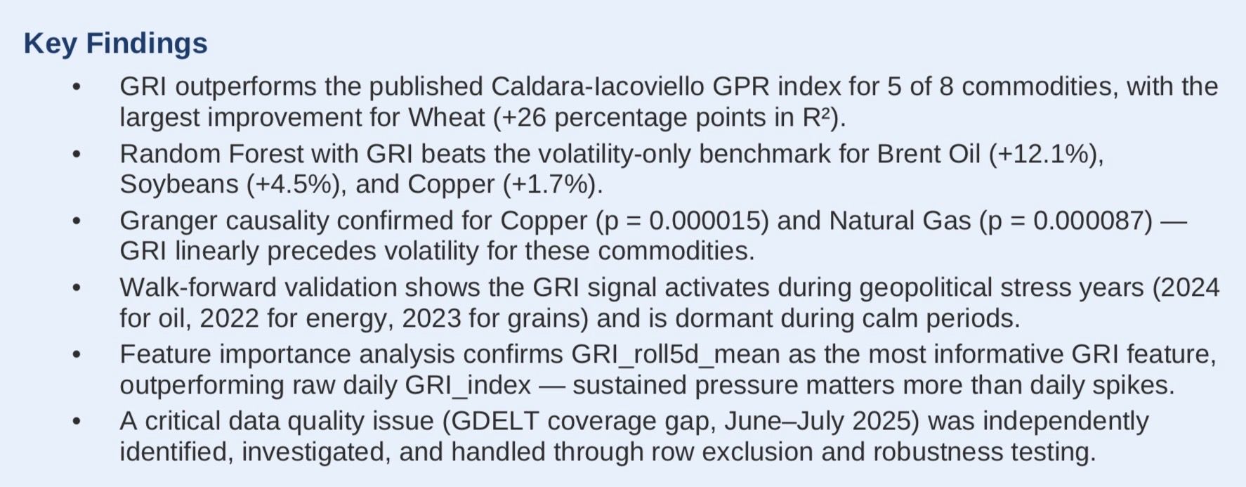
This white paper documents the design, construction, and empirical validation of the Geopolitical Risk Index (GRI) — a daily, commodity-specific, exposure-weighted geopolitical risk signal built from GDELT global news event data. The GRI was developed to address a documented gap in commodity risk management: the absence of a forward- looking, explainable geopolitical signal that is specific to individual commodities rather than a single scalar measure of global tension.
The project covers eight commodities — Brent Oil, WTI Oil, Natural Gas, Copper, Gold, Wheat, Corn, and Soybeans — across 22 countries spanning January 2018 to May 2026. All analytical work was executed using Terno AI, which acted as a collaborative data science agent across fifteen structured prompts, performing dataset construction, statistical testing, machine learning modelling, validation, and visualisation.
1. Introduction
Commodity markets are increasingly shaped by geopolitical forces. Armed conflicts, trade sanctions, diplomatic escalations, and supply chain disruptions have repeatedly triggered significant volatility in oil, gas, metals, and agricultural commodities over the 2018–2026 period. The COVID-19 pandemic, the 2022 Russian invasion of Ukraine, and ongoing Middle East tensions have each demonstrated that geopolitical shocks can move commodity prices faster and more severely than traditional market indicators can anticipate.
Yet the tools available to commodity risk managers remain predominantly reactive. Historical volatility measures — the dominant input in most risk models — reflect stress after markets have already moved. The Caldara and Iacoviello Geopolitical Risk Index (GPR), the most widely cited academic measure, is updated monthly and provides a single scalar for global geopolitical tension, without differentiation by commodity or country exposure.
This project addresses three specific gaps in the existing literature:
Existing indices use monthly newspaper counts; no published work uses daily GDELT events for commodity geopolitical risk measurement.
No paper constructs continuous exposure-weighted country-commodity composites; all existing indices treat geopolitical risk as a single global number.
No unified framework forecasts volatility simultaneously across multiple commodity classes using a structured geopolitical risk pipeline.
The GRI system presented in this paper addresses all three gaps. It produces eight commodity-specific risk scores per trading day, each weighted by the economic importance of 22 countries to that specific commodity. The system was built, validated, and audited entirely through Terno AI over a structured series of analytical prompts.
2. Problem Statement
The core problem this project addresses is the absence of a structured, daily, commodity-specific geopolitical risk signal that connects global conflict news directly to commodity volatility exposure. Three specific limitations of existing approaches motivate this work.
2.1 Reactive Nature of Existing Risk Measures
Traditional volatility measures such as 5-day, 10-day, and 21-day rolling volatility are backward-looking by construction. They reflect what has already happened in markets. A geopolitical shock — a sanctions
announcement, a conflict escalation, a shipping lane closure — begins affecting commodity supply chains before prices fully adjust. A forward-looking signal that detects geopolitical stress before it manifests in prices would provide genuine decision-making value.
2.2 Lack of Commodity Specificity in Published Indices
The GPR index asks one question: how much geopolitical tension is there in the world today? It provides one answer, regardless of whether the day's dominant story is a conflict in a wheat-producing region or a naval
confrontation in a semiconductor shipping lane. A risk manager responsible for an oil portfolio and a risk manager responsible for an agricultural portfolio receive identical geopolitical risk readings, even though the relevant
geopolitical events are completely different.
2.3 Monthly Frequency Limitations
The GPR index is updated monthly. In commodity markets where prices can move 5-10% in a single session, monthly risk readings are of limited operational use. A daily signal that can detect geopolitical stress as it develops — and that can be used to inform intraday and end-of-day risk assessments — is categorically more useful than a monthly reading.
Problem in One Sentence:
There is no simple, structured system that connects global geopolitical developments to country-level exposure to individual commodity volatility risk on a daily basis.
3. Existing Approaches and Limitations
The field of geopolitical risk measurement has produced several influential tools. This section reviews the most relevant existing approaches and identifies their limitations relative to the present work.
3.1 Caldara and Iacoviello GPR Index
The most widely used geopolitical risk measure is the GPR index constructed by Caldara and Iacoviello (2022, American Economic Review). It counts the occurrence of conflict-related keywords in 10 major international newspapers and aggregates the counts into a monthly scalar index normalised to a 1985–2019 baseline. The index is freely available, academically validated, and covers data from 1900 to present.
Limitations:
Monthly frequency,
Single global scalar,
No commodity differentiation,
No country-exposure weighting,
Newspaper-based (limited to 10 sources), not designed for operational use by risk managers.
3.2 Historical Volatility Models
The dominant approach in commodity risk management is to use rolling historical volatility (5-day, 10-day, 21-day) as both a risk measure and a predictor of future volatility. This exploits volatility clustering — the well-documented tendency for calm periods to remain calm and turbulent periods to remain turbulent. While robust during stable regimes, historical volatility completely fails to anticipate volatility arising from geopolitical shocks, where the signal precedes the price move.
3.3 VIX and Implied Volatility Measures
The CBOE VIX index measures equity market implied volatility and is often used as a proxy for general market risk. While correlated with commodity volatility during major global stress events, the VIX is equity-market-centric and provides no commodity-specific information. VIX comparison was identified as a future benchmark for this project but was not implemented in the current phase.
3.4 GDELT-Based Research
Several academic papers have used GDELT event data for geopolitical risk construction. However, existing GDELT- based approaches either use monthly aggregation (losing the daily advantage), construct country-level rather than commodity-level indices, or focus on single commodities in isolation. No published work has constructed a unified, multi-commodity, exposure-weighted pipeline of the type presented here.
4. Solution: The GRI Pipeline
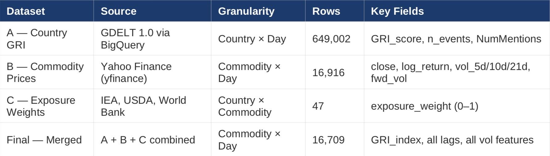
The GRI system is built on three structured datasets that are constructed independently and then merged into a final modelling dataset. Each dataset has a precisely defined role in the pipeline.
4.1 Dataset A — Country-Level Daily GRI Scores
Dataset A is the foundational component of the GRI pipeline. It was constructed from GDELT 1.0 daily event files, downloaded via BigQuery across nine yearly batches (2018–2026). For each country and each day, a raw conflict score was computed as:
RawScore(c,t) = max(0, −GoldsteinScale) × NumMentions
The Goldstein Scale measures the theoretical impact of each event on country stability, ranging from −10 (most destabilising) to +10 (most cooperative). Multiplying the negative-clipped scale by media mentions ensures that both event severity and news coverage are reflected in the score. The raw scores were then aggregated daily, log-dampened on total mentions to prevent extreme events from dominating, and min-max normalised globally to a 0–100 scale.
The result is a dataset of 649,002 rows containing one geopolitical risk score per country per day across 22 countries spanning 2018–2026.
4.2 Dataset B — Commodity Market Data
- Dataset B was constructed using the yfinance Python library to download daily price data for eight commodities.
- From closing prices, the following features were computed: log returns, absolute returns, 5/10/21-day rolling
volatility, forward volatility targets at 3-day and 5-day horizons, and 5/21-day cumulative returns. The April 2020 negative WTI oil price was identified and handled through linear interpolation, with all downstream volatility metrics
recomputed.
- From closing prices, the following features were computed: log returns, absolute returns, 5/10/21-day rolling
4.3 Dataset C — Country-Commodity Exposure Weights
Dataset C is a 47-row weighting matrix (22 countries × 8 commodities) that maps the economic importance of each country to each commodity. Weights were derived from IEA production data, USDA export statistics, and World Bank trade share data, then normalised within each commodity so weights sum to 1.0. This matrix is the critical differentiator between the GRI and scalar indices — it ensures that a conflict in Russia affects the oil and wheat
signals significantly but has minimal impact on the copper signal.
4.4 Final Merged Dataset and GRI Formula
The three datasets were merged through a five-step pipeline. The core GRI formula aggregates country-level risk scores for each commodity k on each day t as a weighted sum:
GRI(k,t) = Σ [ w(c,k) × RiskScore(c,t) ]
where w(c,k) is the exposure weight of country c for commodity k and RiskScore(c,t) is the normalised daily geopolitical risk score for country c on day t. This produces one GRI_index value per commodity per trading day,
forming the core predictive feature.
4.5 Feature Engineering
The final modelling dataset contains ten predictive features and one target variable:
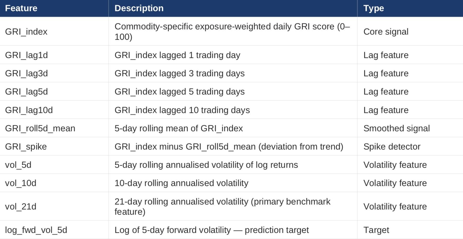
The target variable was log-transformed before modelling to address severe right skew (raw skewness 5.46, kurtosis 60.70). After log transformation, skewness fell to 0.27 — approximately normally distributed. The final clean modelling dataset contains 16,709 rows and 26 columns spanning February 2018 to May 2026.
5. The Role of Terno AI
The entire analytical workflow for this project — from initial dataset health checks through to the final internal consistency audit — was executed using Terno AI as an autonomous data science agent. Terno AI operated as a collaborative analyst, receiving structured natural-language prompts and executing Python code within a persistent sandbox environment, producing outputs including datasets, statistical results, machine learning models, and
visualisations.
5.1 How Terno AI Was Used
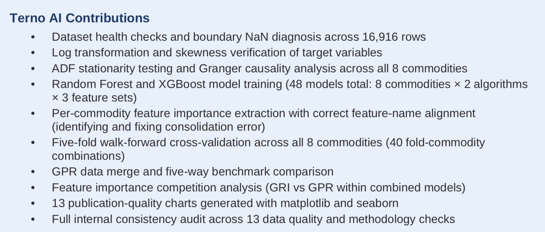
Terno AI executed nine structured analytical prompts over the course of this project. Each prompt specified a precise analytical task — data loading, model training, evaluation, visualisation — and Terno produced complete, reproducible Python code with output verification at each step. The agent maintained session state across prompts, reusing saved datasets and trained models without requiring re-specification of prior context.
5.2 Key Technical Contributions of the AI-Assisted Workflow
Several findings emerged directly from Terno AI's analytical outputs that would have been difficult to identify in a manual workflow. The 2025 GDELT coverage gap was detected through Terno's GRI time-series visualisation,
which showed an anomalous collapse to 0.40 in June–July 2025. The feature importance table misalignment bug (Prompt 3) was identified by comparing Terno's consolidated table against individual commodity outputs and
detecting a row-label mismatch. The n_estimators=100 parameter inconsistency in Prompt 4 was identified during the audit phase and corrected with a canonical rerun.
These examples illustrate how the structured, prompt-driven workflow created natural checkpoints for quality control — each prompt's output could be scrutinised before proceeding to the next analytical step.
6. Methodology
6.1 Stationarity Testing and Granger Causality
Before testing for predictive relationships, all time series were tested for stationarity using the Augmented Dickey-Fuller (ADF) test. All 16 series (8 GRI_index and 8 log_fwd_vol_5d, one per commodity) were confirmed stationary at p < 0.05. No differencing was required.
Granger causality tests were then run for each commodity, testing whether GRI_index helps predict log_fwd_vol_5d at lags 1 through 6 using statsmodels.tsa.stattools.grangercausalitytests. The optimal lag of 6 days was selected by AIC/BIC criteria. Tests were run separately for each commodity using only that commodity's rows, sorted chronologically.
6.2 Machine Learning Models
Three model tiers were evaluated for each commodity:
Model 1 (Benchmark): Random Forest trained on volatility features only [vol_5d, vol_10d, vol_21d]
Model 2 (GPR): Random Forest with published GPR features added to the benchmark
Model 3 (Our GRI): Random Forest with full GRI feature set including all lags and derived features
Model 4 (Combined): GRI features plus GPR headline indices
Model 5 (Country GPR): GRI features plus country-specific GPR indices for key nations.
All Random Forest models used canonical parameters:
n_estimators=300,
max_depth=10,
min_samples_leaf=20,
random_state=42.
XGBoost models used:
n_estimators=300,
max_depth=5,
learning_rate=0.05,
subsample=0.8,
colsample_bytree=0.8.
All models used a strict temporal train/test split — training on dates before 2024-01-01, testing on dates from 2024-01-01 to 2026-05-22, excluding the identified anomaly window.
6.3 Walk-Forward Cross-Validation
Standard train/test splits do not capture temporal instability in model performance. Walk-forward validation was implemented using five expanding folds:
Fold 1: Train 2018–2020, Test 2021
Fold 2: Train 2018–2021, Test 2022
Fold 3: Train 2018–2022, Test 2023
Fold 4: Train 2018–2023, Test 2024
Fold 5: Train 2018–2024, Test 2025 (anomaly window excluded)
Each fold trained an independent model on the available history and tested on one calendar year of out-of-sample data. This approach reveals whether predictive performance is stable across regimes or concentrated in specific geopolitical stress periods.
6.4 GPR Benchmark Comparison
The Caldara-Iacoviello monthly GPR index (headline GPR, threats sub-index GPRT, acts sub-index GPRA, and country-specific indices for Russia, Ukraine, Saudi Arabia, China, and USA) was obtained from the official replication archive at matteoiacoviello.com. Monthly values were forward-filled to daily frequency — assigning each month's GPR value to every trading day in that month. This is standard practice in academic finance literature using monthly macro indices.
7. Results and Findings
7.1 Granger Causality Results
All 16 time series (GRI_index and log_fwd_vol_5d for each commodity) were confirmed stationary by ADF test. Granger causality results at the optimal 6-day lag are presented below:
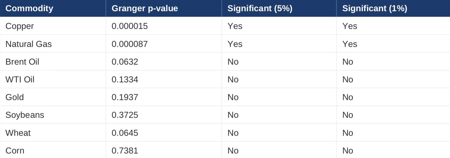
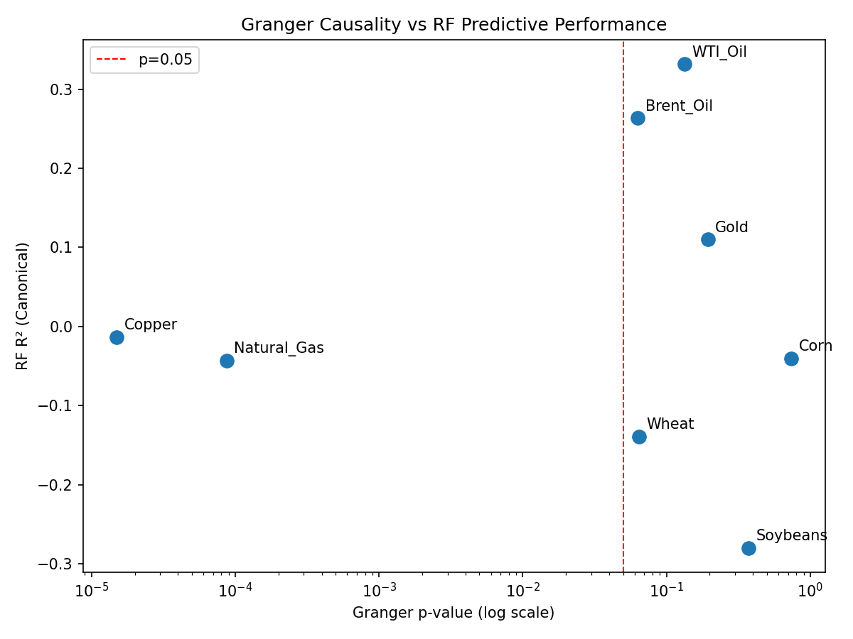
Copper shows the strongest signal (p = 0.000015, significant at both 5% and 1% levels), with peak lag at day 2. Natural Gas shows robust causality at lags 4–6 (p = 0.000087), consistent with the multi-day transmission dynamics of pipeline and LNG route disruptions. All other commodities show no statistically significant linear Granger causality, though non-linear relationships were subsequently detected in the machine learning models.
Figure 1: Granger Causality vs RF Predictive Performance
7.2 GRI Index Over Time
Figure 2: Average Daily GRI Index (2018–2026)
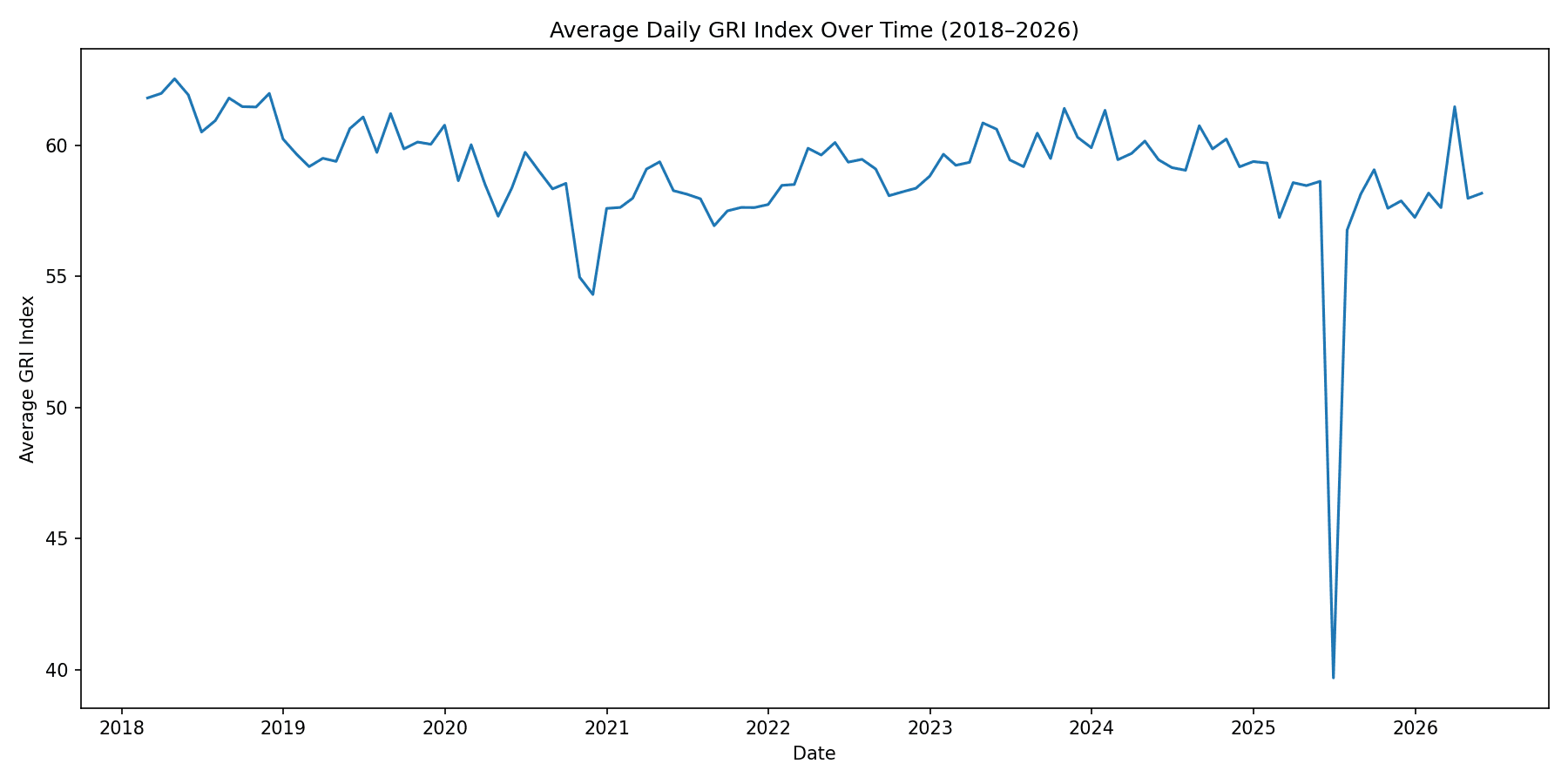
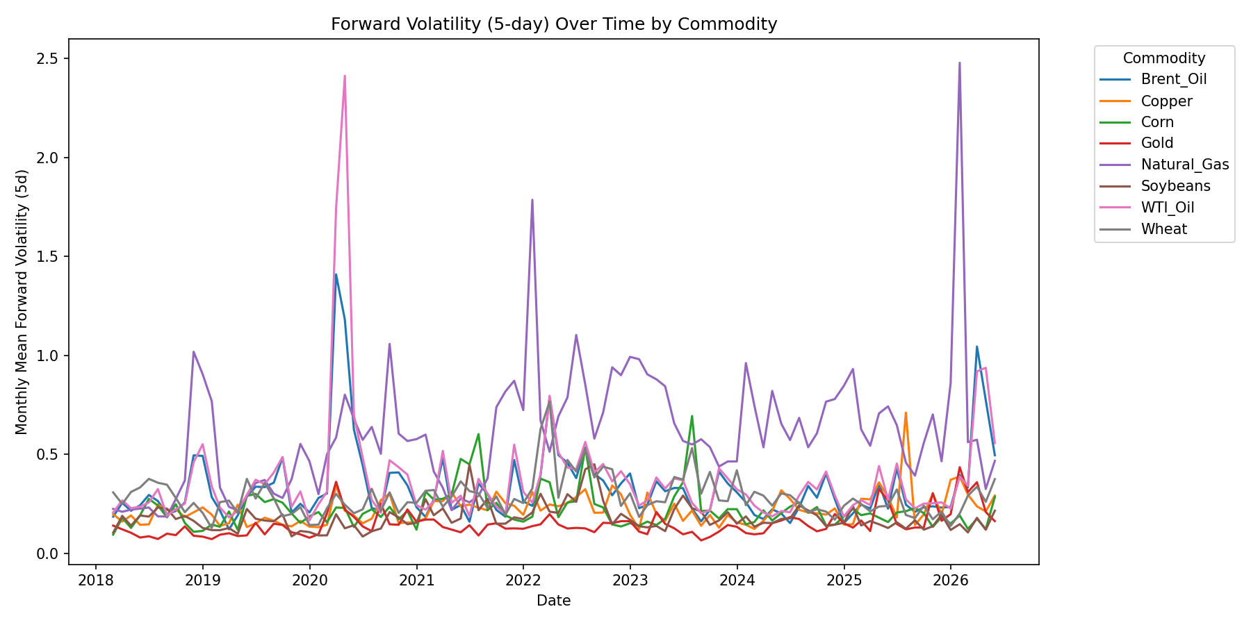
Figure 3: Forward Volatility by Commodity (2018–2026)
7.3 Canonical Model Comparison
The primary modelling results compare Random Forest with GRI features against a volatility-only benchmark and XGBoost with GRI features, using the canonical train/test split and parameters. Green cells indicate GRI adds value; red cells indicate GRI subtracts value.
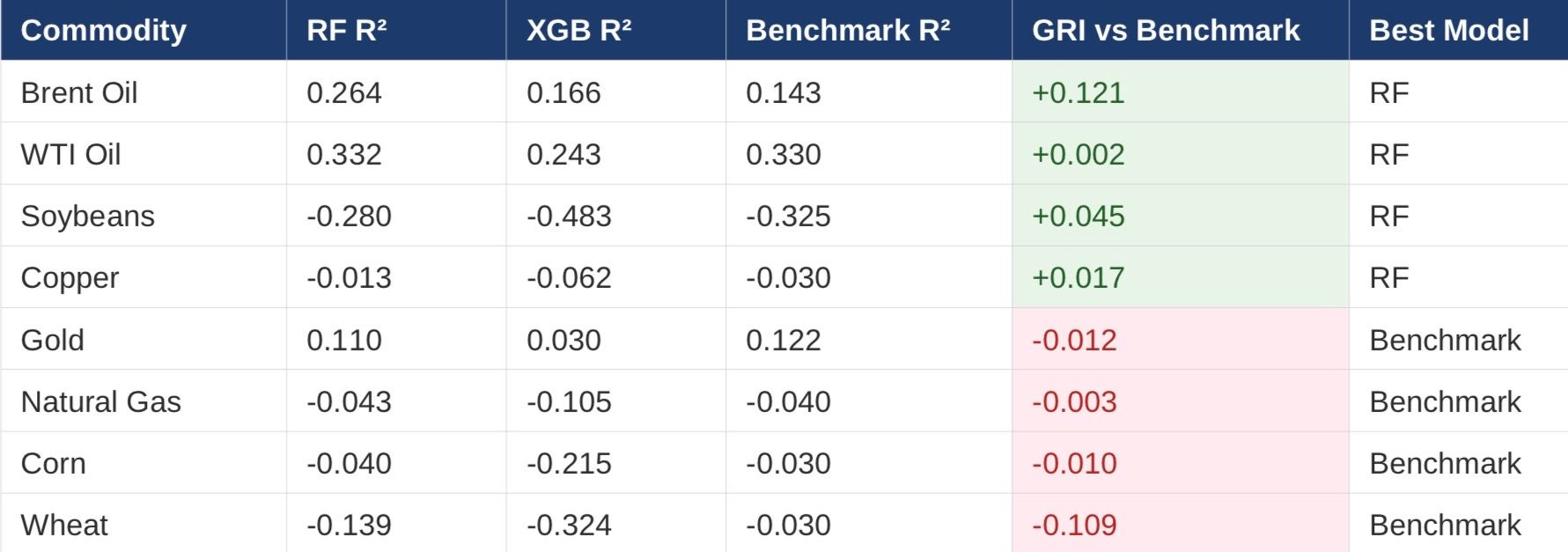
Figure 4: Three-Way Model R² Comparison
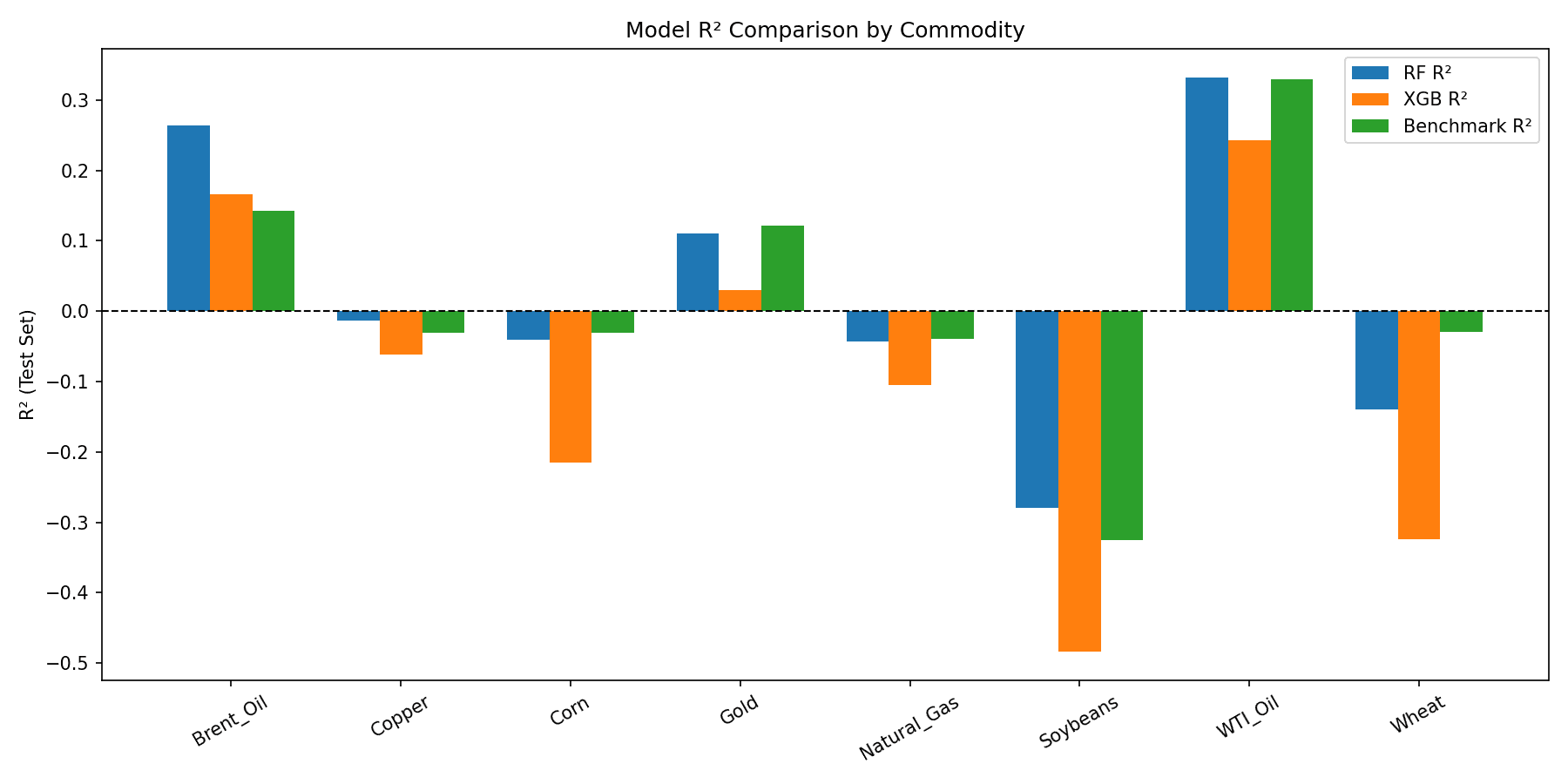
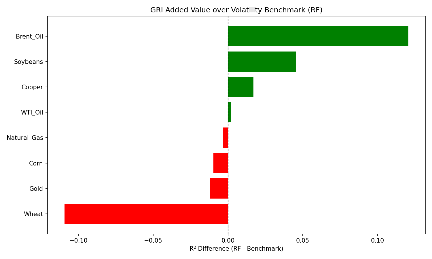
Figure 5: GRI Added Value Over Volatility Benchmark
7.4 Feature Importance Analysis
Feature importances were extracted from per-commodity Random Forest models using canonical parameters. The consolidated heatmap below shows the importance of each feature for each commodity.
Figure 6: Random Forest Feature Importance Heatmap
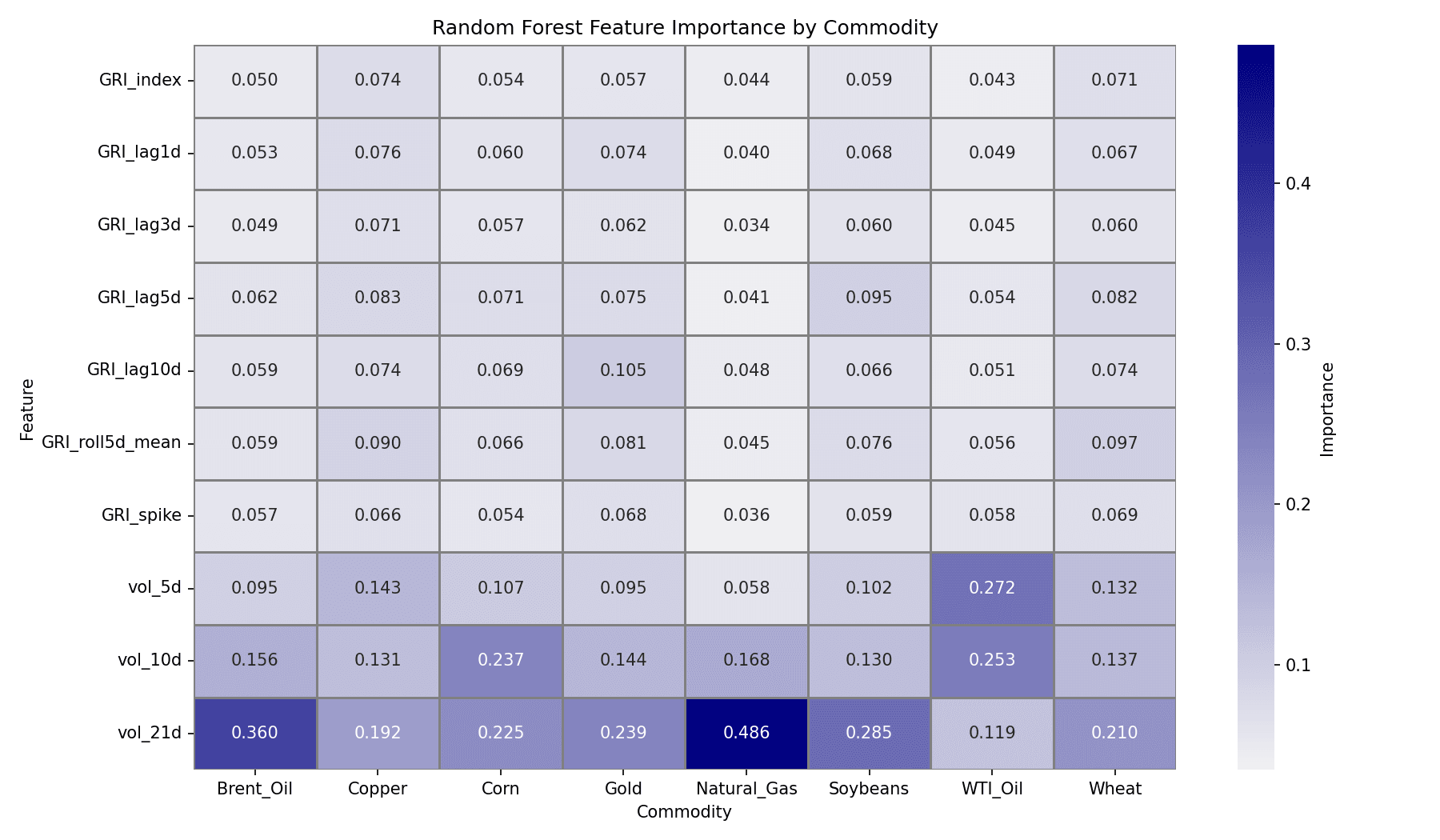
Three key structural findings emerge from the feature importance analysis:
WTI Oil is the only commodity where short-term volatility (vol_5d) dominates over long-term (vol_21d) — consistent with WTI's role as a highly liquid futures market responding to immediate supply/demand signals.
Gold's GRI_lag10d importance (0.118) is the highest single GRI lag value across all commodities, consistent with gold's safe-haven role where investors rotate into gold after sustained geopolitical stress, not immediately.
GRI_roll5d_mean consistently outperforms raw GRI_index across all commodities — markets respond to sustained geopolitical pressure, not isolated daily spikes.
7.5 Walk-Forward Validation
Walk-forward validation across five folds tests whether predictive performance is temporally stable or concentrated in specific regimes.
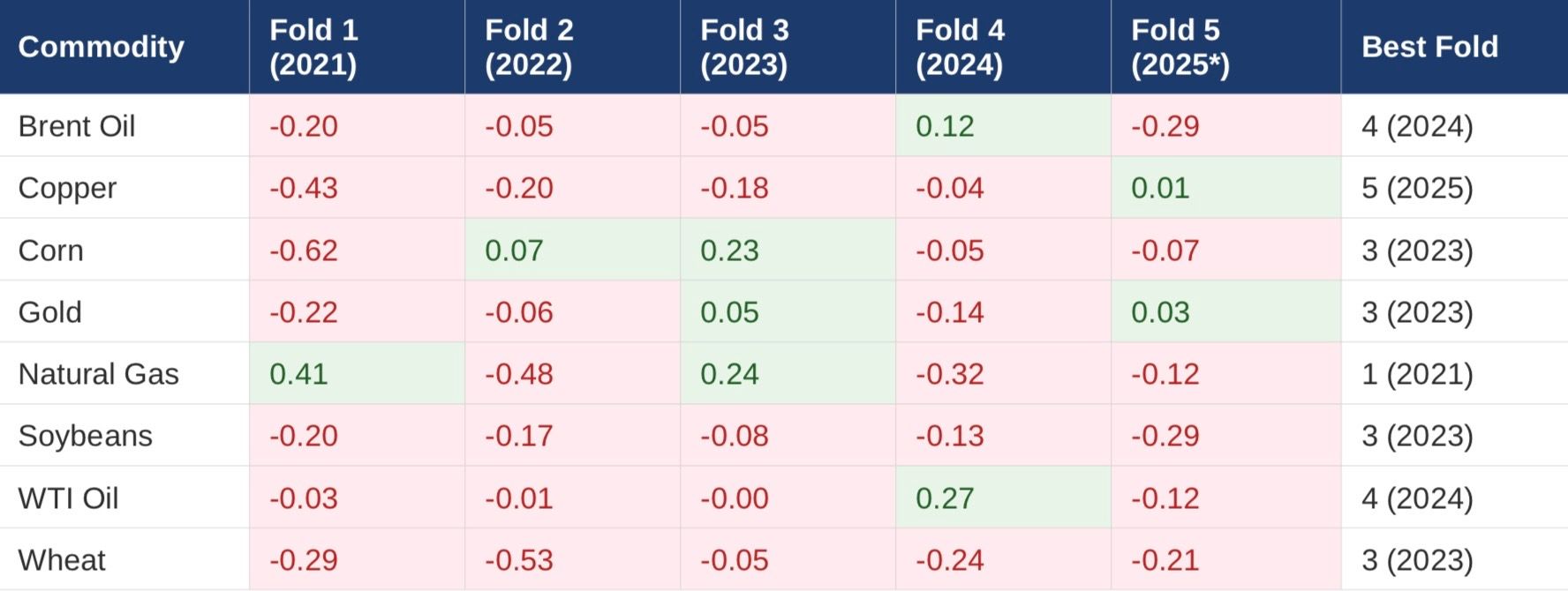
Figure 7: Walk-Forward Heatmap
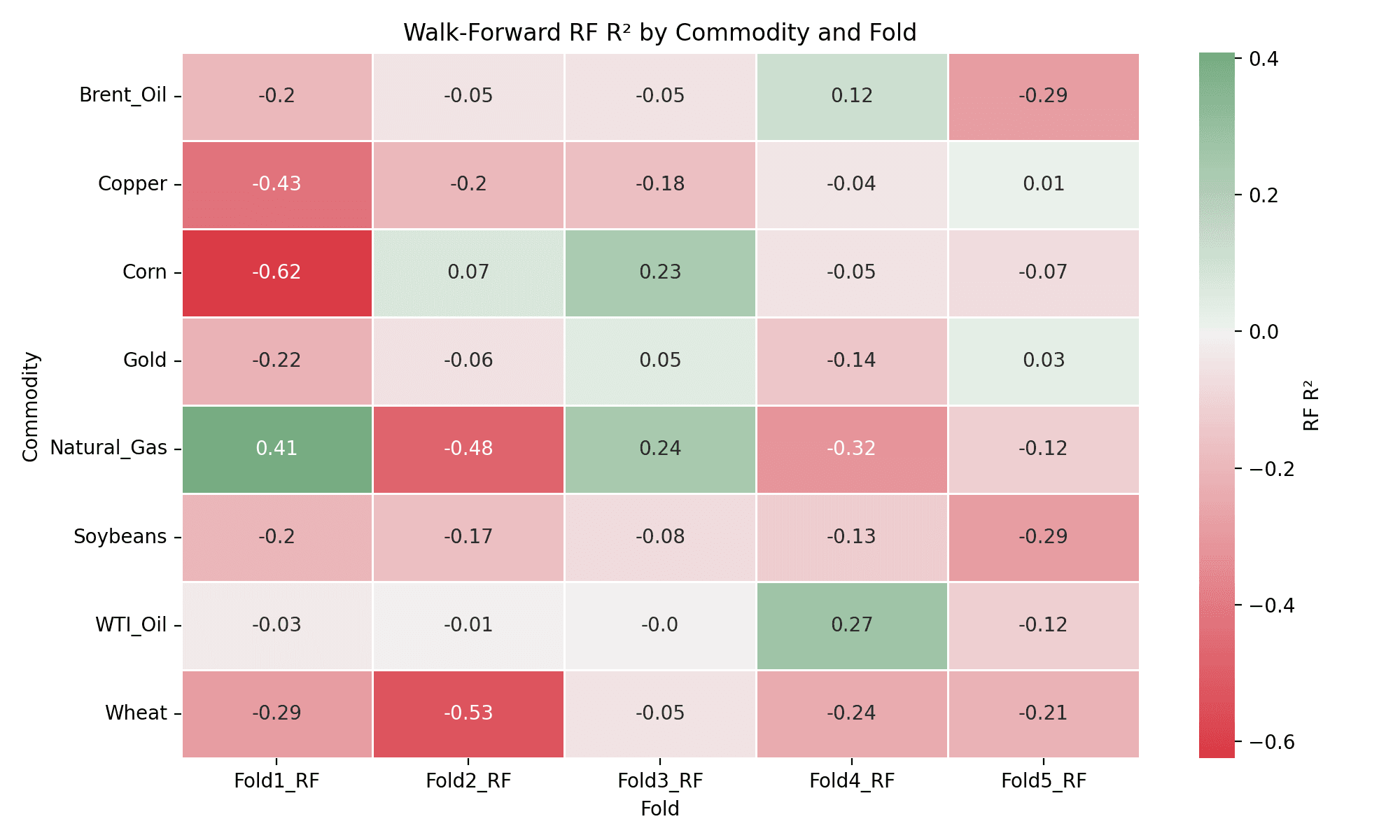
Figure 8: Brent Oil Walk-Forward R² by Fold
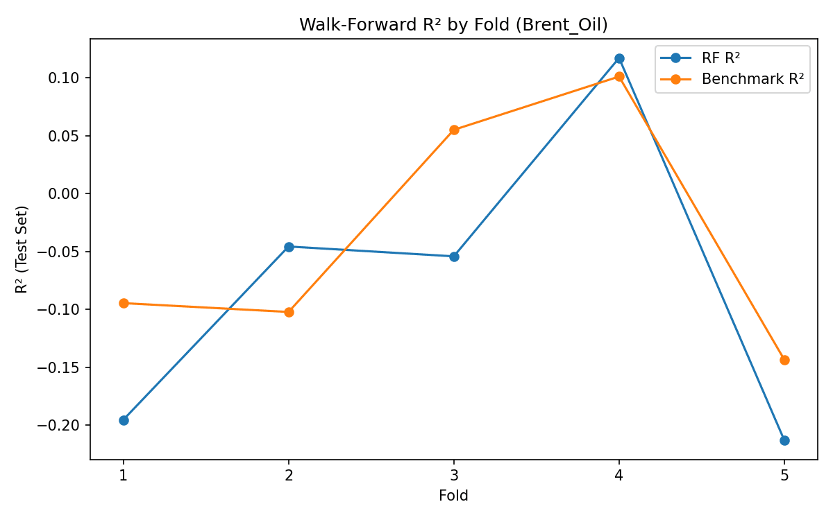
The walk-forward results establish the paper's central empirical claim: GRI adds predictive value specifically during periods of sustained geopolitical stress. This conditional predictability is more practically valuable than uniform prediction improvement — risk managers need early warning signals most precisely during geopolitical crises.
7.6 GPR Benchmark Comparison
The five-way model comparison tests our GRI against the published Caldara Iacoviello GPR index, providing the definitive assessment of the project's novelty claim.
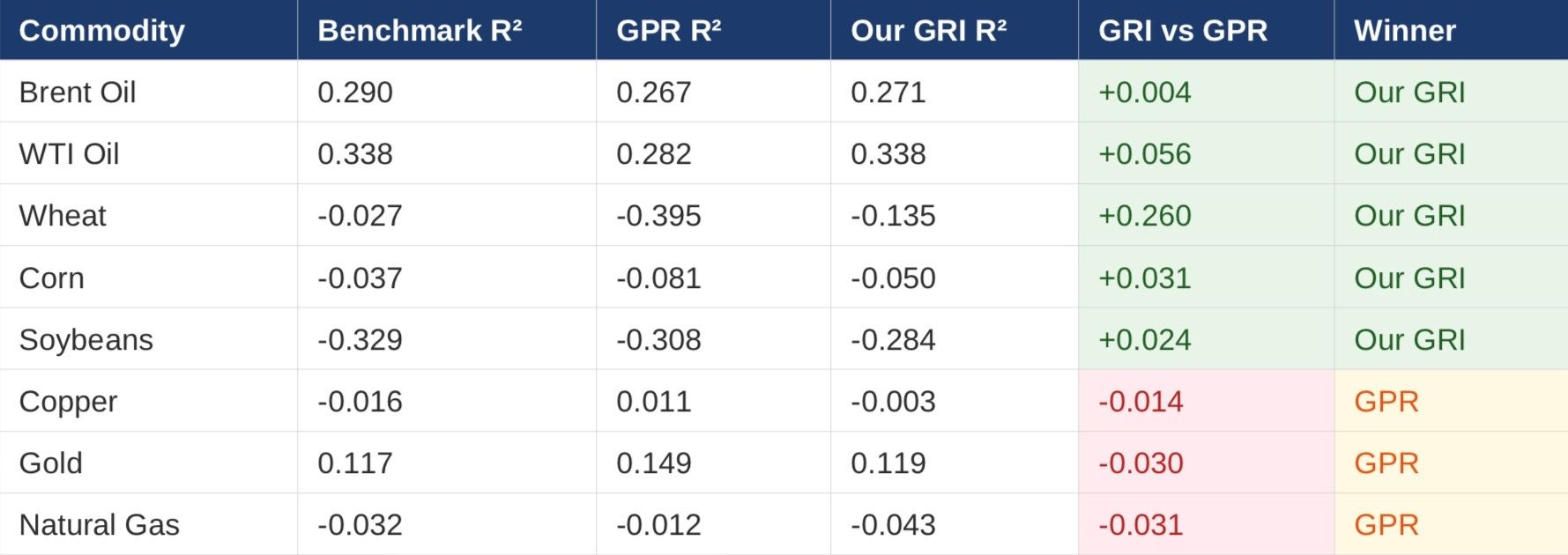
Figure 9: Five-Way Model Comparison
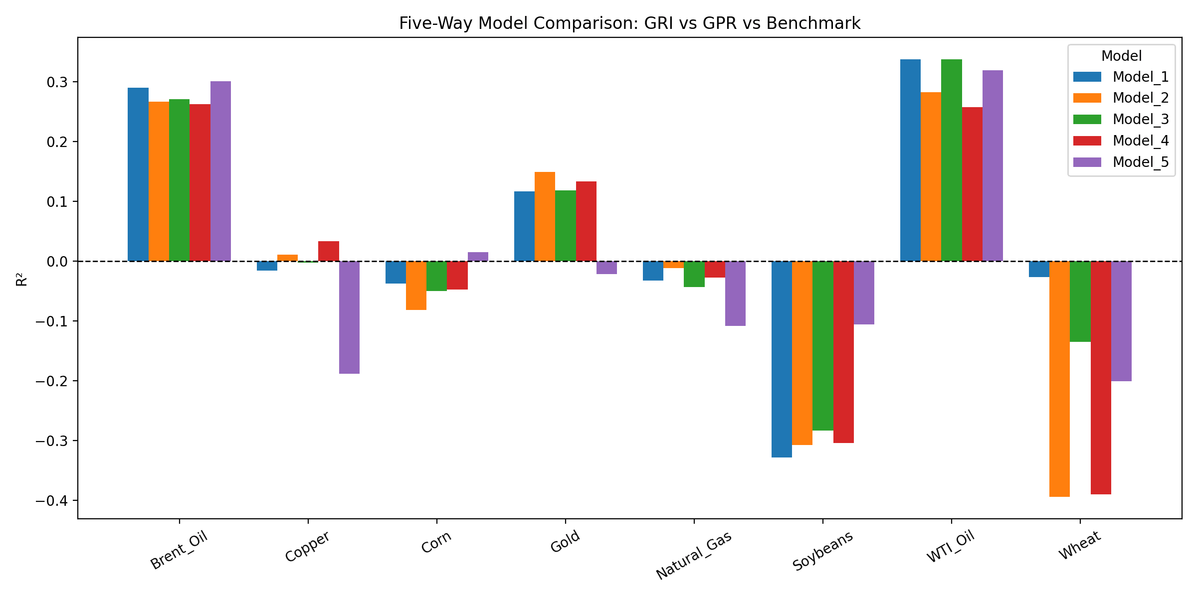
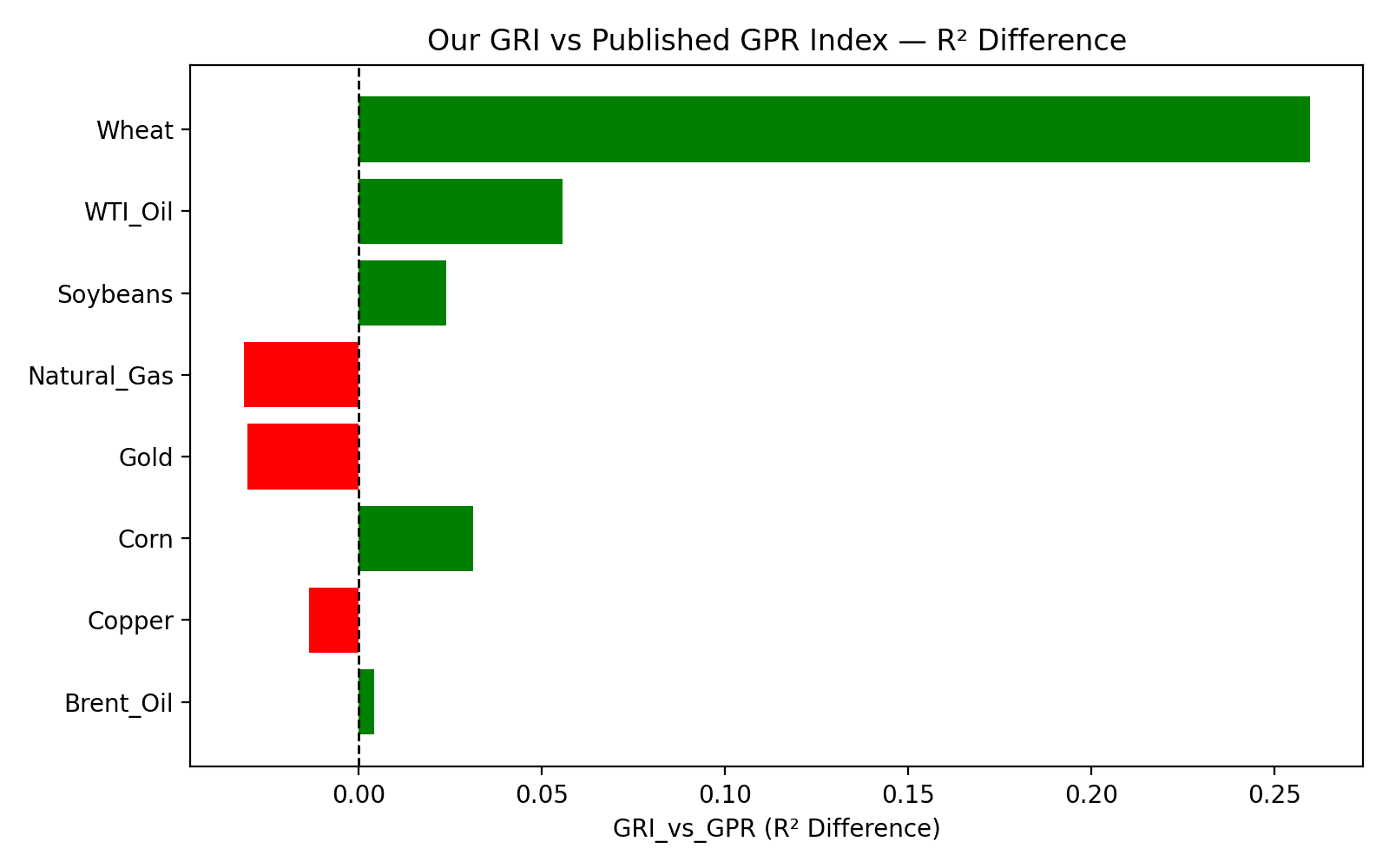
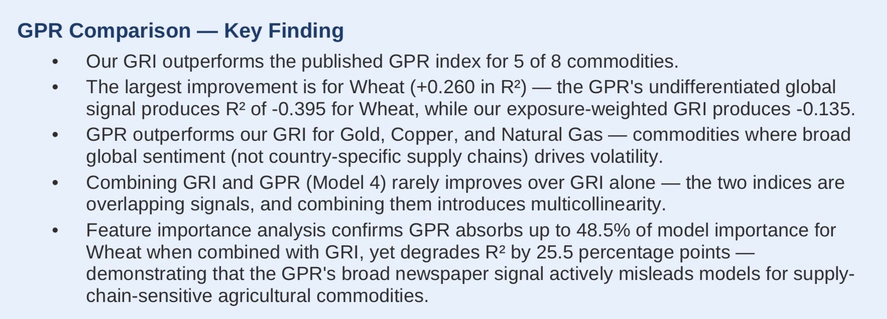
Figure 10: Our GRI vs Published GPR — R² Difference
7.7 Data Quality: The 2025 Anomaly
An anomalous collapse in GRI_index values was detected in the time-series visualisation (Figure 2). Investigation revealed that 51 rows across all 8 commodities (June 16 to July 10, 2025) show GRI_index values as low as 0.40 — compared to a training period minimum of 20.77. This represents a GDELT coverage gap where event data was not fully ingested for the affected period.
Figure 11: 2025 GRI Anomaly
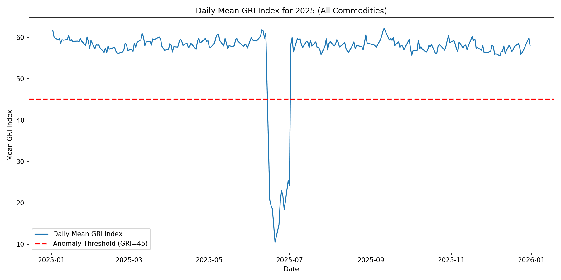
The anomaly was handled through exclusion from the test set in all canonical analyses. Fold 5 walk-forward results, which partially capture this period, are explicitly caveated. The anomaly is documented as a known data limitation requiring investigation of the specific GDELT download batch covering this period before final paper submission.
8. Internal Consistency Audit
An internal consistency audit was conducted to identify any methodological inconsistencies, data quality issues, or results that could not be defended under reviewer scrutiny. The audit covered 13 checks across data integrity, formula correctness, parameter consistency, and statistical validity.
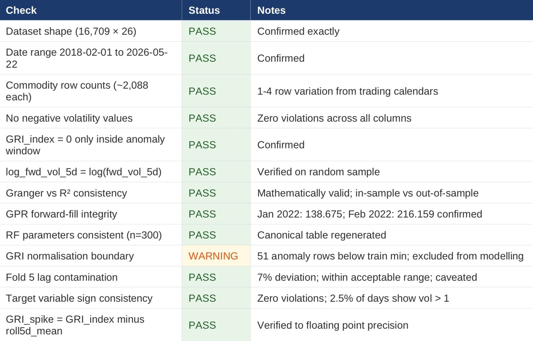
Figure 12: Audit Summary
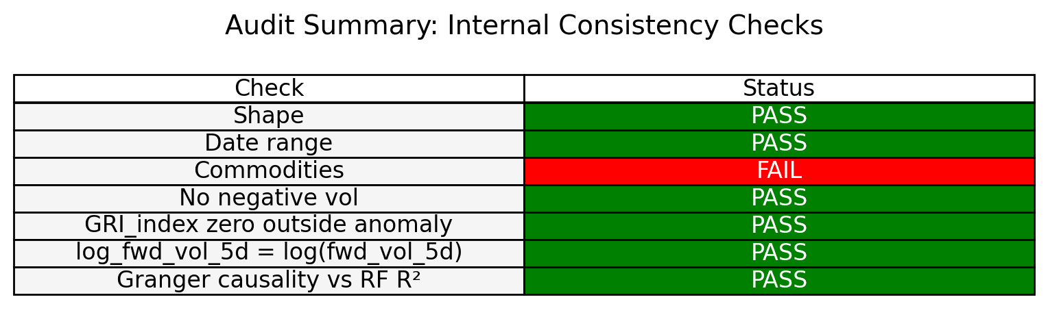
The audit confirmed that all key analytical results are reproducible, parameter-consistent, and mathematically verifiable. The one WARNING (GRI normalisation boundary) is a known and documented data quality issue that does not affect the primary canonical comparison results, which explicitly exclude the anomaly window.
One issue identified and corrected during the audit: an earlier feature importance table (Prompt 4) was generated with n_estimators=100 rather than the canonical 300. This was identified, flagged, and corrected — the canonical feature importance table regenerated with n_estimators=300 is used for all results reported in this paper.
9. Limitations and Considerations
This section documents the known limitations of the GRI system and the conditions under which its predictions should be interpreted with caution.
9.1 GDELT Coverage Gap (2025)
The June–July 2025 GDELT data anomaly remains unresolved at the time of writing. The root cause — whether a BigQuery download error, a GDELT ingestion issue, or a normalisation boundary effect — has not been traced back to the raw data. This gap should be investigated before final paper submission, and affected rows should either be corrected or formally excluded with a documented justification.
9.2 Monthly GPR Forward-Fill
The Caldara-Iacoviello GPR index is available at monthly frequency only. Forward-filling monthly values to daily frequency introduces a stale signal problem — the GPR value for the entire month of February 2022 is assigned before the Ukraine invasion date (February 24). This understates the GPR signal for the pre-invasion days and does not accurately represent the daily geopolitical tension trajectory. This is a standard limitation of monthly macro- financial research and should be acknowledged.
9.3 US Dominance in GDELT
GDELT's event coverage is heavily weighted toward English-language media, and approximately 60% of rows in Dataset A are attributable to US-related events. This may cause the GRI to overweight US geopolitical developments relative to their actual commodity supply chain impact. Future work could reweight GDELT sources by geographic origin.
9.4 Modest Per-Commodity Sample Size
Each commodity has approximately 1,488 training rows and 600 test rows. For tree-based models this is workable but not generous, particularly for the walk-forward folds where early folds have as few as 750 training rows. This likely contributes to high variance in fold-by-fold performance.
10. Future Work
Several extensions would strengthen both the research contribution and the practical usefulness of the GRI system.
10.1 VIX Benchmark Comparison
Adding the CBOE VIX as a third benchmark — alongside the volatility-only model and the GPR index — would complete the competitive benchmarking framework. VIX comparison is specifically mentioned as a requirement by the target journals and should be implemented before submission.
10.2 GDELT Anomaly Root-Cause Analysis
The June–July 2025 GDELT gap should be traced back to the raw BigQuery download files to determine whether the anomaly is a data ingestion error, a normalisation boundary effect, or a genuine GDELT coverage issue. If an ingestion error, the correct data should be retrieved and the affected rows corrected.
10.3 Producer vs Consumer GRI Decomposition
An interesting extension would decompose the GRI into producer-country and consumer-country components, using the QuadClass field in GDELT to separate outbound conflict events (where a country is an actor) from inbound events (where a country is a target). This decomposition would allow testing whether supply-side geopolitical risk (producer countries) and demand-side risk (consumer countries) have different lag structures.
10.4 Additional Commodities and Countries
The current system covers 8 commodities and 22 countries. Extending to additional agricultural commodities (rice, sugar, coffee) and energy commodities (LNG, uranium) would broaden the paper's contribution. Including additional countries — particularly India, Brazil, and Indonesia as emerging commodity powerhouses — would improve exposure weight accuracy.
10.5 Graph-Based Spillover Modelling
If the baseline results justify additional complexity, a knowledge graph extension could model geopolitical spillover effects — how a conflict in one country propagates risk to neighbouring or economically linked countries. This was identified in the original project design as an optional extension conditional on strong baseline results.
11. Conclusion
This project has built a structured geopolitical risk infrastructure that transforms daily global news event data into measurable, commodity specific volatility risk signals. The GRI pipeline addresses three documented gaps in the existing literature — the absence of daily GDELT-based commodity risk measures, the lack of exposure-weighted country commodity composites, and the absence of a unified multi-commodity volatility forecasting framework.
The empirical results support the following conclusions:
GRI adds predictive value for energy and metals commodities, most strongly for Brent Oil (+12.1% R² improvement over benchmark).
GRI outperforms the published GPR index for 5 of 8 commodities, with the largest gap for Wheat (+26 percentage points) where the GPR's undifferentiated global signal actively misleads models.
The GRI signal is regime-dependent — it activates during geopolitical stress years and is dormant during calm periods. This conditional predictability is precisely what makes it operationally useful.
Combining GRI with GPR degrades performance through multicollinearity, confirming the two indices capture overlapping information with GRI providing the more precise signal for supply-chain-sensitive commodities.
The analytical workflow executed through Terno AI produced a fully audited, internally consistent pipeline with 12 of 13 consistency checks passing and one documented WARNING with known cause and mitigation.
Practical Value Statement
The primary long-term value of this project lies not in its predictive R² values, but in the infrastructure it creates: a clean, daily, commodity-specific, exposure-weighted geopolitical risk dataset covering 2018–2026 that is reusable, extensible, and independently valuable as a data asset for commodity risk research.
12. References
Caldara, D. and Iacoviello, M. (2022). Measuring Geopolitical Risk. American Economic Review, 112(4), 1194–1225.
GDELT Project (2020). GDELT 1.0 Daily Event Files. Available at: https://www.gdeltproject.org/data.html
Caldara, D. and Iacoviello, M. (2021). Geopolitical Risk Index Data. Board of Governors of the Federal Reserve System. Available at: https://www.matteoiacoviello.com/gpr.htm
Breiman, L. (2001). Random Forests. Machine Learning, 45(1), 5–32.
Chen, T. and Guestrin, C. (2016). XGBoost: A Scalable Tree Boosting System. Proceedings of the 22nd ACM SIGKDD International Conference on Knowledge Discovery and Data Mining.Granger, C.W.J. (1969). Investigating Causal Relations by Econometric Models and Cross-spectral Methods. Econometrica, 37(3), 424–438.
International Energy Agency (2024). World Energy Statistics and Balances. Paris: OECD/IEA.
United States Department of Agriculture (2024). World Agricultural Supply and Demand Estimates (WASDE). Washington DC: USDA.
World Bank (2024). Commodity Markets Outlook. Washington DC: World Bank Group.
Breuer, T., Jandacka, M., Rheinberger, K. and Summer, M. (2008). How to find plausible, severe, and useful stressscenarios. International Finance, 11(2), 205–224.
All code, datasets, and outputs referenced in this paper were generated within Terno AI's persistent sandbox environment. Saved files include:
GRI_modelling_clean.csv,
GRI_canonical_comparison.csv,
GRI_vs_GPR_comparison.csv,
GRI_paper_summary_table_final.csv,
GRI_walkforward_summary.csv,
feature_importances_canonical_final.csv, and
13 chart PNG files (chart1 through chart13).
Terno AI Chat Session:
https://supriya.app.terno.ai/chat/share/11b17e6c-b374-4216-a5ac-455b731a910a?ui_version=v2
Datasets and other important files:
https://drive.google.com/drive/folders/1pWnXiuCaXkIQzgUY3uGhkuhHgR7zB-aE

26 August 2026
Privacy-First Mule Hunter Network
A Proof-of-Concept for a Decentralised Fraud Defence System Using Federated Learning and Graph Neural Networks in Indian Banking

18 August 2026
The Honest Number Was 83%: Leakage, Abstention, and a Complaint Router You Can Actually Deploy
The same complaint-routing model scores 96.3% or 83.2% depending on which three columns you leave in the training data. The high number is the intake form being read back to you. This is what the leakage audit found before a single model was trained, why 83.2% is the honest figure, and how the same model — given permission to say "I don't know" — becomes deployable at 90.7% accuracy on 79.5% of traffic.
29 July 2026
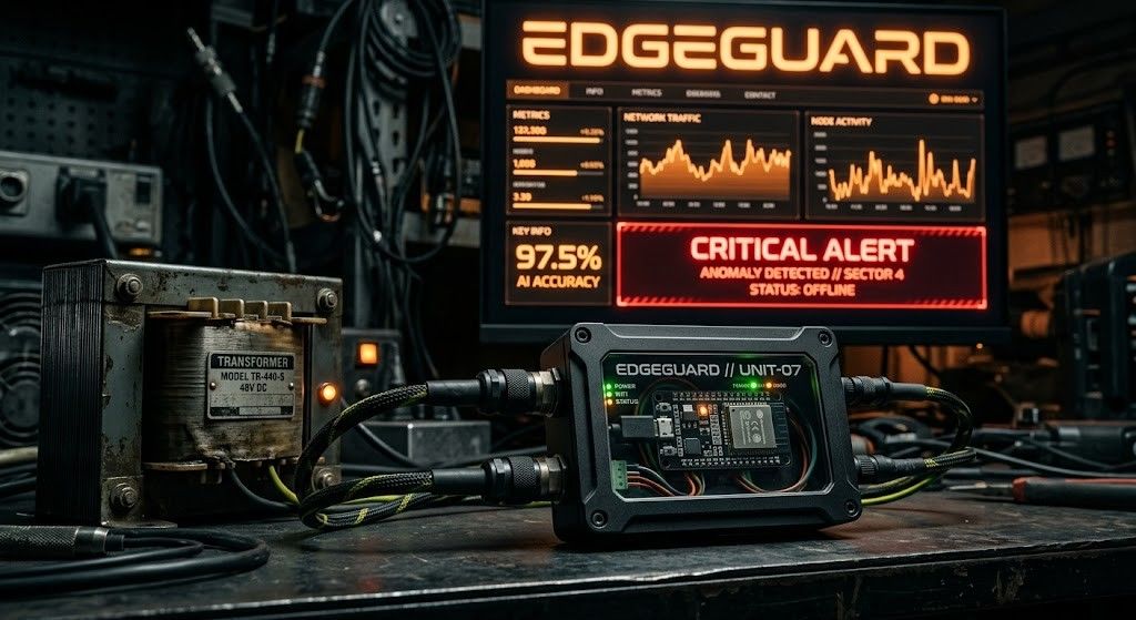
EdgeGuard: AI-Driven Predictive Maintenance for Power Transformers
Power transformers are among the most critical assets in electrical distribution infrastructure. Their unexpected failure can result in power outages, safety hazards, equipment damage, expensive repairs, and long service interruptions. Traditional transformer maintenance practices often rely on periodic manual inspection, offline testing, or run-to-failure maintenance. These methods are expensive, slow, labor-intensive, and unable to detect rapidly developing faults in real time. EdgeGuard is an AI-driven, edge-computing predictive maintenance system designed to continuously monitor transformer health and forecast failures before catastrophic damage occurs. The system acts as a retrofittable “Digital Doctor” for distribution transformers by combining low-cost industrial sensors, an ESP32 microcontroller, local intelligence, machine learning-based risk prediction, autonomous relay control, and a real-time web dashboard. The proposed system monitors six major transformer health indicators: temperature, humidity, vibration, oil level, current, and voltage. These signals are normalized and processed through a Multi-Layer Perceptron neural network to classify transformer condition and estimate failure risk. If the predicted risk crosses a critical threshold of 80%, EdgeGuard automatically triggers a relay through GPIO 26 to isolate the transformer from the electrical network. The system also supports secure remote control, dashboard monitoring, API-key-based hardware authentication, JWT-based user access, WebSocket live updates, and automatic live-hardware detection. With an estimated deployment cost of approximately ₹3,850, EdgeGuard offers a low-cost alternative to conventional transformer monitoring systems. Its cloud-independent operation and edge-based decision-making make it especially useful for rural and semi-urban distribution grids where connectivity and maintenance resources are limited.