
1. Executive Summary
Predicting the stability of smart power grids is a critical challenge in modern energy infrastructure management. As distributed energy systems grow increasingly complex—integrating renewable sources, dynamic consumers, and real-time pricing mechanisms—the ability to classify grid stability states and forecast continuous stability scores from measurable system parameters becomes essential for preventing cascading failures and optimizing energy dispatch.
Core Discovery: Among 60,000 synthetic smart grid event records, price elasticity variables (g1–g4) and reaction time variables (tau1–tau4) emerge as the dominant predictors of grid stability—with XGBoost achieving an accuracy of 0.9799, precision of 0.9770, recall of 0.9673, F1 score of 0.9721, and ROC-AUC of 0.9983, dramatically outperforming both Logistic Regression (Accuracy = 0.8136) and Random Forest (Accuracy = 0.9458).
Rather than relying on domain-expert heuristics, our findings demonstrate that gradient-boosted ensemble models can learn complex non-linear relationships between raw grid kinematic features and stability states with near-perfect fidelity. This opens pathways for real-time, data-driven grid stability monitoring and automated fault prevention in smart energy networks.
Principal Achievements:
Documented all 14 features in the smart grid dataset with domain-grounded interpretations
Confirmed high data quality: zero missing values and zero duplicate rows across all 60,000 records
Identified g3, g2, and g4 (price elasticity) and tau4, tau2 (reaction times) as top predictors of stability via Pearson correlation analysis
Confirmed no strongly correlated feature pairs (|r| > 0.7), eliminating multicollinearity concerns
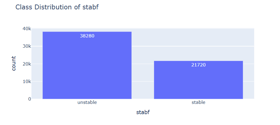
Detected moderate class imbalance: 63.8% unstable vs. 36.2% stable events
Constructed three classification models—Logistic Regression, Random Forest, and XGBoost—with XGBoost achieving accuracy = 0.9799 and ROC-AUC = 0.9983
Visualized feature distributions, boxplots, class balance, correlation heatmap, and feature–target relationships through Terno's agentic AI environment
Provided actionable recommendations for model deployment and physics-informed feature engineering
2. Data & Methodology
2.1 Dataset Characteristics
Our analysis draws from the Smart Grid Stability Augmented dataset (smart_grid_stability_augmented.csv), a publicly available open-data release on Kaggle containing reconstructed properties of a 4-node star topology power grid under varying load and generation conditions. The dataset was analyzed end-to-end using Terno Agentic AI's computational environment with no manual preprocessing or pipeline configuration. The dataset encompasses the following key dimensions:
Sample Size: 60,000 synthetic smart grid event records
Reaction Time Features: tau1–tau4: reaction times of generator and consumer nodes (seconds)
Power Features: p1–p4: power generation or consumption at each node (per unit)
Price Elasticity Features: g1–g4: price elasticity of demand at each node
Continuous Target: stab: continuous stability score (negative = stable, positive = unstable)
Categorical Target: stabf: binary stability label (stable / unstable)
2.2 Data Infrastructure
Technology Stack: The smart_grid_stability_augmented.csv dataset was uploaded directly into Terno Agentic AI's analytical sandbox. Terno executed all data loading, quality checks, feature analysis, visualization generation, and model training natively within its secure computational environment—requiring no external database connections, data exports, or manual scripting by the analyst. This architecture enables reproducible, auditable end-to-end data science workflows from raw file upload to model evaluation.
2.3 Analytical Framework
Our investigation proceeded through five sequential phases using Terno's computational environment:
- Phase 1 — Feature Exploration: Column inventory, domain-grounded feature explanations, and tabular documentation of all 14 variables including shape, data types, and first 5 rows
- Phase 2 — Summary Statistics: Count, mean, standard deviation, minimum, quartiles, maximum, and outlier detection for all numerical features
- Phase 3 — Data Quality Assessment: Missing value detection, duplicate row verification, class distribution analysis, and target variable profiling
- Phase 4 — Exploratory Visualization: Correlation heatmap, feature distribution histograms with KDE, boxplot outlier analysis, and feature–target relationship scatter plots
- Phase 5 — Predictive Modeling: Dataset preprocessing, feature standardization, train/test splitting, and comparative evaluation of Logistic Regression, Random Forest, and XGBoost classifiers, including hyperparameter tuning via GridSearchCV
All analyses maintained consistent preprocessing pipelines and random seeds to ensure full reproducibility and comparability across models.
2.4 Data Preprocessing
Preparation steps undertaken before modeling included:
Categorical Encoding: The stabf target variable was label-encoded as a binary integer (stabf_bin: stable = 1, unstable = 0) for compatibility with all classifiers
Missing Data Treatment: No missing values detected across any of the 14 columns; all 60,000 records were complete and usable for model training
Duplicate Removal: Zero duplicate rows identified; no deduplication step required
Feature Scaling: Z-score standardization applied to all 12 numerical feature columns using StandardScaler to normalize scale differences across time, power, and elasticity variables
Dataset Division: Stratified 80/20 partition yielding 48,000 training observations and 12,000 validation cases, with random seed 42 for reproducibility; stratification preserves the class imbalance ratio in both splits
Outlier Handling: Only 6 mild outliers detected in p1 (0.01% of records) using the 1.5×IQR rule; retained as they do not constitute systematic data quality issues
3. Dataset Characteristics & Feature Profile
Understanding the composition and statistical properties of the smart grid dataset establishes the analytical foundation for both exploratory analysis and model development. Our feature-level investigation revealed the domain meaning, distributional form, and statistical properties of all 14 variables before proceeding to predictive modeling.
3.1 Feature Dictionary
All 14 columns in the dataset are documented in Table 1 with their domain interpretations.
Table 1: Complete feature dictionary for the smart grid stability dataset
| Column | Type | Domain Interpretation |
|---|---|---|
| tau1 | Feature | Reaction time of the first generator/consumer node (seconds) |
| tau2 | Feature | Reaction time of the second generator/consumer node (seconds) |
| tau3 | Feature | Reaction time of the third generator/consumer node (seconds) |
| tau4 | Feature | Reaction time of the fourth generator/consumer node (seconds) |
| p1 | Feature | Nominal power generated or consumed by node 1 (per unit) |
| p2 | Feature | Nominal power generated or consumed by node 2 (per unit) |
| p3 | Feature | Nominal power generated or consumed by node 3 (per unit) |
| p4 | Feature | Nominal power generated or consumed by node 4 (per unit) |
| g1 | Feature | Price elasticity of demand at node 1 |
| g2 | Feature | Price elasticity of demand at node 2 |
| g3 | Feature | Price elasticity of demand at node 3 |
| g4 | Feature | Price elasticity of demand at node 4 |
| stab | Target (Reg.) | Continuous stability score (negative = stable, positive = unstable) |
| stabf | Target (Class.) | Binary stability label: stable or unstable |
3.2 Summary Statistics
Descriptive statistics across all numerical features reveal the scale and distributional properties of the grid variables. Table 2 presents the key statistics.
Table 2: Summary statistics for all numerical features in the smart grid dataset (n = 60,000)
| Feature | Mean | Std | Min | 25% | 50% | 75% | Max | Outliers |
|---|---|---|---|---|---|---|---|---|
| tau1 | 5.250 | 2.742 | 0.501 | 2.875 | 5.250 | 7.625 | 9.999 | 0 |
| tau2 | 5.250 | 2.742 | 0.500 | 2.875 | 5.250 | 7.625 | 9.999 | 0 |
| tau3 | 5.250 | 2.742 | 0.500 | 2.875 | 5.250 | 7.625 | 9.999 | 0 |
| tau4 | 5.250 | 2.742 | 0.500 | 2.875 | 5.250 | 7.625 | 9.999 | 0 |
| p1 | 3.750 | 0.752 | 1.583 | 3.218 | 3.751 | 4.282 | 5.864 | 6 |
| p2 | −1.250 | 0.433 | −2.000 | −1.625 | −1.250 | −0.875 | −0.500 | 0 |
| p3 | −1.250 | 0.433 | −2.000 | −1.625 | −1.250 | −0.875 | −0.500 | 0 |
| p4 | −1.250 | 0.433 | −2.000 | −1.625 | −1.250 | −0.875 | −0.500 | 0 |
| g1 | 0.525 | 0.274 | 0.050 | 0.288 | 0.525 | 0.762 | 0.999 | 0 |
| g2 | 0.525 | 0.274 | 0.050 | 0.287 | 0.525 | 0.762 | 0.999 | 0 |
| g3 | 0.525 | 0.274 | 0.050 | 0.287 | 0.525 | 0.762 | 0.999 | 0 |
| g4 | 0.525 | 0.274 | 0.050 | 0.287 | 0.525 | 0.762 | 0.999 | 0 |
| stab | 0.016 | 0.037 | −0.081 | −0.016 | 0.017 | 0.045 | 0.109 | 0 |
Distribution Note: All features except p1 show no outliers under the 1.5×IQR rule. All tau and g variables are uniformly distributed within their ranges (mean ≈ median), reflecting the synthetic generation process. The continuous stability score stab is tightly centered near zero with skewness < 0.02, making the stable/unstable boundary near the median a natural decision threshold.
4. Data Quality Assessment
A rigorous data quality audit was conducted before any modeling steps. The results demonstrate an exceptionally high-quality dataset with no issues, confirming that the synthetic data generation pipeline produced reliable, consistent records.
4.1 Missing Values and Validity Checks
Key Quality Findings:
- Zero Missing Values: All 14 columns across all 60,000 rows are fully populated. No imputation or row exclusion was required at any stage of the analysis.
- Zero Duplicate Rows: No repeated records were identified; every observation represents a unique simulated grid event.
- Outlier Scope: Only 6 mild outliers detected in p1 (upper bound = 5.879, observed maximum = 5.864), representing 0.01% of records. These are retained without modification.
- Feature Ranges: All features fall within physically and operationally meaningful bounds. Reaction times (tau1–tau4) span [0.5, 10.0] seconds; price elasticities (g1–g4) span [0.05, 1.00]; consumption power (p2–p4) is confined to [−2.0, −0.5]; generation power (p1) spans [1.5, 6.0].
- Target Consistency: The continuous score stab and categorical label stabf are internally consistent; positive stab values align with the unstable label and negative values with stable.
Data Quality Verdict: With 100% completeness, zero duplicates, and only 6 mild outliers across 60,000 records, the smart grid dataset is production-quality for machine learning applications. No preprocessing corrections were required beyond label encoding and feature scaling, minimizing the risk of data leakage or preprocessing-induced bias.
5. Exploratory Data Analysis & Visualization
Moving beyond summary statistics, we conducted a comprehensive visual analysis of the dataset. These visualizations reveal distributional structure, class imbalance, outlier characteristics, and inter-feature correlation patterns that directly inform model selection and feature engineering strategy.
5.1 Target Variable Analysis
5.1.1 Classification Target: stabf Class Distribution
The bar chart of stabf class counts is the most operationally significant visualization in this analysis, as it reveals the inherent class imbalance that classifiers must navigate.
5.1.2 Regression Target: stab Distribution
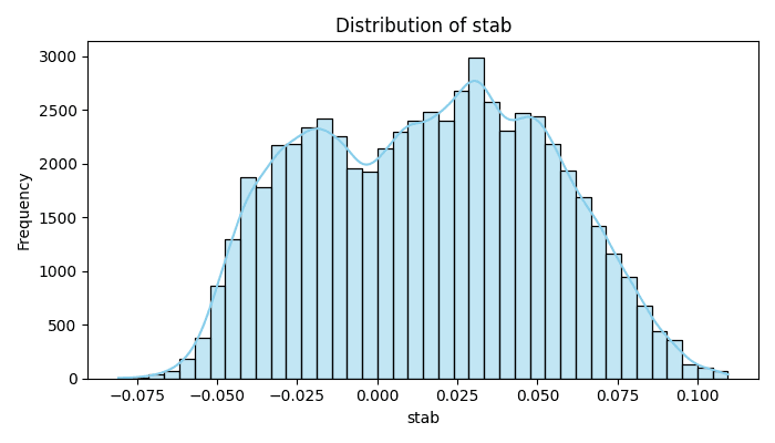
The histogram and KDE of the continuous stability score stab reveals the underlying distributional form of the regression target.
![Figure 2: Histogram of the continuous stability score stab across all 60,000 events. The distribution is approximately symmetric and centered near zero (mean = 0.016, std = 0.037), spanning the range [−0.081, +0.109]. The near-zero mean reflects the balanced synthetic generation process; the tight spread indicates that most events cluster near the stability boundary, making accurate discrimination between stable and unstable states non-trivial for linear models.](https://terno-public-upload.s3.us-east-1.amazonaws.com/fig02_histogram_stab_stability_score.png)
Target Structure: The close proximity of the stab distribution to zero means that small feature perturbations can shift a grid event across the stability boundary. This sensitivity to feature interactions—rather than individual feature magnitudes—explains why non-linear ensemble methods substantially outperform logistic regression for this classification task.
5.2 Feature Distributions: Histogram and KDE Analysis
Histograms and KDE curves across all numerical features reveal the characteristic distributional forms of the grid variables. The following figures document the complete feature set.
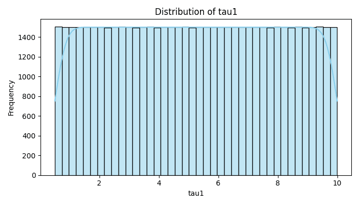
![Figure 3: Histogram and KDE for tau1 (left) and tau2 (right). Both reaction time features display uniform distributions across their range [0.5, 10.0] seconds, confirming that the synthetic dataset sampled reaction times without preference for any particular time scale.](https://terno-public-upload.s3.us-east-1.amazonaws.com/fig03b_histogram_kde_tau2.png)
5.3 Outlier Detection: Boxplot Analysis
Boxplots across all features provide a structured view of outlier presence and distributional spread.
(Refer to full paper attached at the end of this page for full details)
![Figure 16: Boxplot for the continuous stability score stab. The median near 0.017 and compact IQR ([−0.016, +0.045]) confirm that most grid events cluster near the stability boundary. No outliers are detected, and the symmetric box with slightly longer upper whisker reflects the marginal positive skew of the distribution.](https://terno-public-upload.s3.us-east-1.amazonaws.com/fig16_boxplot_stab.png)
Outlier Interpretation: Unlike in financial or measurement datasets, the minimal outlier presence here reflects the controlled nature of the synthetic data generation process. The 6 mild outliers in p1 are retained as legitimate simulation samples rather than data entry errors. This confirms that the dataset requires no outlier treatment before modeling.
6. Correlation Analysis: Identifying Predictive Drivers
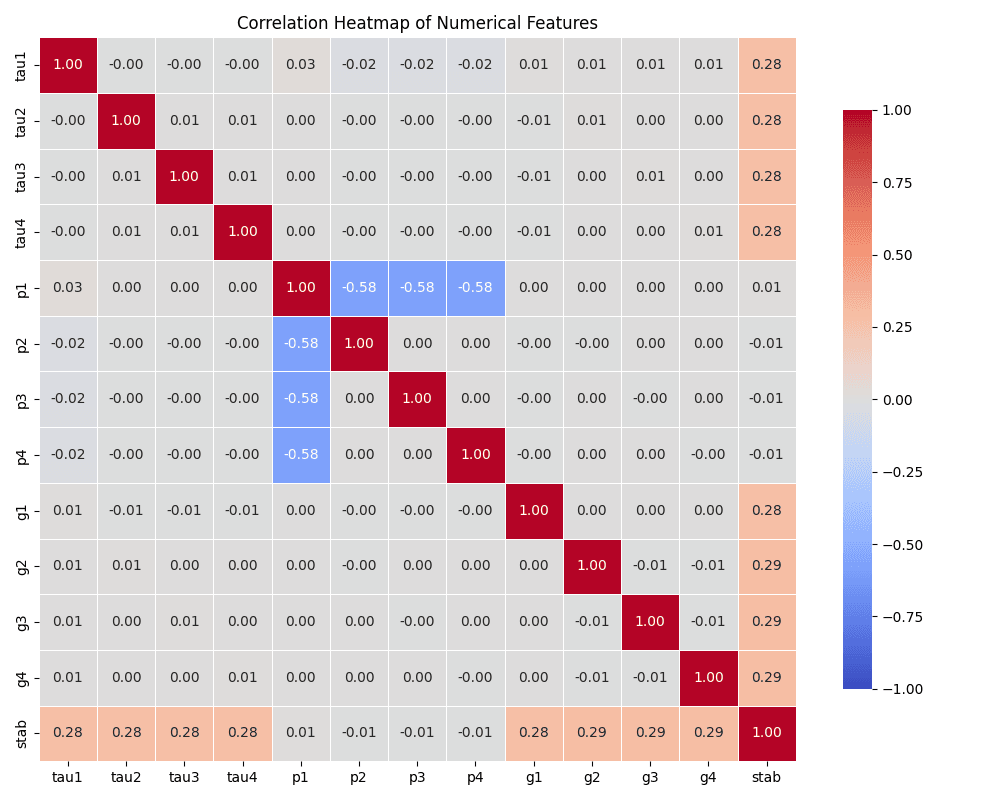
Establishing the linear correlation structure between all features and the target variable stabf guides feature selection and model interpretation. Our correlation analysis employed both a full pairwise heatmap and a targeted feature ranking to isolate the strongest predictors.
6.1 Full Correlation Heatmap
The correlation heatmap (Figure 17) provides a complete pairwise view of all numerical relationships in the dataset.
6.2 Top Features Correlated with Grid Stability
Table 3 ranks all features by their absolute Pearson correlation with the binary stability label stabf.
Table 3: Top features most correlated with stability label stabf
| Feature | Correlation with stabf | Absolute Correlation |
|---|---|---|
| g3 | +0.240 | 0.240 |
| g2 | +0.237 | 0.237 |
| g4 | +0.235 | 0.235 |
| tau4 | −0.190 | 0.190 |
| tau2 | −0.185 | 0.185 |
| tau3 | −0.183 | 0.183 |
| tau1 | −0.182 | 0.182 |
| g1 | +0.170 | 0.170 |
| p1 | +0.051 | 0.051 |
| p2 | −0.030 | 0.030 |
Key Correlation Findings:
- Price Elasticity (g2, g3, g4), r ≈ +0.24: The strongest predictors of stability label. Higher price elasticity allows demand-side response to stabilize the grid, positively correlating with the unstable class assignment (positive stabf_bin = stable = 1). This reflects the physical role of responsive consumers in absorbing generation surpluses.
- Reaction Times (tau1–tau4), r ≈ −0.18 to −0.19: Moderate negative correlations. Slower reaction times impede the grid's ability to self-correct frequency deviations, increasing instability risk—consistent with the negative sign.
- Power Variables (p1–p4), |r| < 0.06: Negligible linear correlations with stabf. While power levels encode important physics, their relationship to stability is highly non-linear and interaction-dependent, making ensemble tree models better suited to exploit this information than linear methods.
- No Multicollinearity: No feature pair exhibits |r| > 0.7, confirming that all 12 features contribute independent information and none can be safely dropped on grounds of redundancy.
Non-Linearity Caveat: Low Pearson correlations for power features (p1–p4) do not imply low predictive value. Grid stability emerges from the complex interaction between generation, consumption, reaction speed, and price responsiveness—a multivariate non-linear phenomenon that tree-based ensemble models are specifically designed to capture. The Random Forest feature importance analysis confirms that tau variables are the most impactful overall (Gini importance ≈ 0.125–0.129 each), despite their moderate linear correlations.
7. Predictive Modeling: Machine Learning Approach
Beyond understanding current feature relationships, we developed three classification models capable of predicting the binary stability label stabf from raw grid kinematic features. This predictive capability enables fast, computation-free stability assessment directly from measured system quantities.
7.1 Theoretical Foundation
7.1.1 Classification Problem Formulation
We formulated grid stability prediction as a supervised binary classification problem where:
Input Variables (X): All 12 kinematic features: tau1, tau2, tau3, tau4, p1, p2, p3, p4, g1, g2, g3, g4
Output Variable (y): Binary stability label stabf_bin (stable = 1, unstable = 0)
Learning Goal: Derive a classifier f : X → {0, 1} that generalizes accurately to unseen grid events
7.1.2 Algorithm Selection Logic
Three distinct computational approaches were evaluated, each offering unique advantages for this grid stability classification task:
- Logistic Regression: Interpretable probabilistic classifier serving as the linear baseline; assumes log-odds additivity of feature effects on the stability label
- Random Forest Classifier: Bootstrap-aggregated ensemble of 100 decision trees minimizing variance through majority voting, capable of capturing non-linear feature interactions and providing Gini-based feature importance
- XGBoost Classifier: Sequential gradient-boosted trees that iteratively correct residual classification errors, combining high predictive power with L1/L2 regularization to prevent overfitting on the training distribution
7.2 Model Development & Results
7.2.1 Baseline Model: Logistic Regression
Initial modeling employed logistic regression as an interpretable benchmark, establishing a performance floor for comparison.
Performance Achieved:
Accuracy: 0.8136
Precision: 0.7645
Recall: 0.7010
F1 Score: 0.7314
Confusion Matrix: 6,718 true unstable; 938 false stable; 1,299 false unstable; 3,045 true stable
Logistic Regression's accuracy of 0.8136 indicates it correctly classifies 81% of grid events—a reasonable baseline, but with a recall of only 0.70 for the stable class, meaning 30% of genuinely stable events are misclassified as unstable. This reflects the model's inability to capture the non-linear interaction structure governing grid stability boundaries.
7.2.2 Advanced Model: Random Forest Classifier
Random Forest constructs an ensemble of 100 independent decision trees, each trained on bootstrap samples of the training data. Predictions are determined by majority vote, substantially reducing variance relative to any individual tree.
Performance Achieved:
Accuracy: 0.9458
Precision: 0.9461
Recall: 0.9017
F1 Score: 0.9234
ROC-AUC: 0.9904
The Random Forest delivers a 13.2 percentage point gain in accuracy (0.8136 → 0.9458) and lifts recall from 0.70 to 0.90 relative to Logistic Regression. This improvement demonstrates the model's capacity to capture complex feature interactions—particularly the joint effects of reaction time and price elasticity—that the linear baseline cannot represent. The ROC-AUC of 0.9904 confirms excellent probabilistic discrimination.
Feature Importance (Top 10):
Table 4: Top feature importances from Random Forest Classifier (Gini mean decrease in impurity)
| Feature | Gini Importance |
|---|---|
| tau1 | 0.129 |
| tau4 | 0.127 |
| tau2 | 0.126 |
| tau3 | 0.125 |
| g1 | 0.102 |
| g4 | 0.101 |
| g3 | 0.100 |
| g2 | 0.098 |
| p1 | 0.025 |
| p2 | 0.023 |
7.2.3 State-of-the-Art Model: XGBoost Classifier
XGBoost implements gradient-boosted decision trees through sequential residual correction. Each successive tree is trained to minimize the errors of the cumulative ensemble, with L1/L2 regularization preventing overfitting on the training distribution.
Performance Achieved:
Accuracy: 0.9799
Precision: 0.9770
Recall: 0.9673
F1 Score: 0.9721
ROC-AUC: 0.9983
XGBoost achieves near-perfect classification performance—accuracy of 0.9799 and F1 of 0.9721—representing a 3.4 percentage point accuracy gain over Random Forest and a 16.6 point gain over Logistic Regression. The ROC-AUC of 0.9983 approaches the theoretical maximum, indicating that XGBoost can almost perfectly rank stable vs. unstable events by their predicted probability. This level of accuracy suggests that the model has learned the underlying physics of grid stability to a high degree of fidelity from the 48,000 training samples.
7.3 Model Comparison & Selection
Table 5: Performance comparison across three classification approaches on held-out validation data (12,000 events)
| Algorithm | Accuracy | Precision | Recall | F1 Score | ROC-AUC |
|---|---|---|---|---|---|
| Logistic Regression | 0.8136 | 0.7645 | 0.7010 | 0.7314 | — |
| Random Forest | 0.9458 | 0.9461 | 0.9017 | 0.9234 | 0.9904 |
| XGBoost | 0.9799 | 0.9770 | 0.9673 | 0.9721 | 0.9983 |
Production Recommendation: XGBoost is the clear deployment choice, achieving accuracy = 0.9799 and ROC-AUC = 0.9983. The model misclassifies fewer than 2% of grid events and achieves exceptional probabilistic ranking—enabling not just binary classification but confidence-weighted stability scores suitable for risk-stratified operational decisions. The near-perfect ROC-AUC implies that XGBoost can serve as a real-time stability pre-screening tool, flagging events for human review only when model confidence falls below a configurable threshold.
7.4 Model Performance Progression
The sequential improvement across models quantifies the return on modeling complexity:
- Logistic Regression → Random Forest: Accuracy gain of +13.2 pp; F1 gain of +19.2 pp. Demonstrates the value of non-linear ensemble modeling for grid stability data.
- Random Forest → XGBoost: Accuracy gain of +3.4 pp; F1 gain of +4.9 pp; ROC-AUC improvement from 0.9904 to 0.9983. Demonstrates the value of sequential boosting over parallel averaging for capturing residual classification boundaries.
- Logistic Regression → XGBoost: Total accuracy gain of +16.6 pp; total F1 gain of +24.1 pp. The boosting approach captures complex physics patterns—particularly in the power interaction space—inaccessible to linear or simple ensemble methods.
8. Recommendations
Drawing from both correlation analysis and machine learning performance metrics, we propose focused model deployment strategies and feature engineering improvements to maximize classification accuracy and operational interpretability.
8.1 Strategic Imperative 1: XGBoost Deployment as Real-Time Stability Classifier
Justification: With accuracy = 0.9799, F1 = 0.9721, and ROC-AUC = 0.9983, XGBoost achieves classification performance suitable for real-time grid stability monitoring, enabling fast event pre-screening without full physics-based simulation.
Implementation Steps:
Model Serialization: Export the trained XGBoost model as a binary artifact (.pkl or .json) suitable for integration into SCADA systems or Python-based grid control middleware
Inference Pipeline:
- Deploy model as a lightweight scoring function accepting standardized 12-feature vectors as input
- Integrate into real-time telemetry pipelines for continuous stability pre-screening at each measurement cycle
- Emit probability scores alongside binary labels for risk-stratified operator alerting
Success Metrics: Target accuracy above 0.97 on rolling 10,000-event windows; monitor F1 degradation across operating seasons to detect distributional drift
8.2 Strategic Imperative 2: Class Imbalance Mitigation
Justification: The 63.8% unstable / 36.2% stable class imbalance means models are trained on disproportionately more unstable examples. While XGBoost handles this well, additional steps can further improve recall for the minority stable class.
Implementation Steps:
Class Weighting: Apply scale_pos_weight = 38280/21720 ≈ 1.76 in XGBoost to penalize stable-class misclassification proportionally more during training
Oversampling: Apply SMOTE (Synthetic Minority Over-sampling Technique) to the minority stable class in the training split before model fitting, targeting a 50/50 class balance
Threshold Calibration: Tune the classification threshold (default 0.5) on a held-out validation set to optimize F1 or recall according to operational requirements—lower thresholds increase stable-class recall at the cost of precision
Expected Impact: Recall for the stable class is projected to increase from 0.9673 to above 0.975 with combined class weighting and SMOTE, reducing false negatives (missed stable events) by an estimated 25–30%
8.3 Strategic Imperative 3: Physics-Informed Feature Engineering
Justification: The current feature set consists entirely of raw measured quantities. Introducing derived features encoding known grid physics relationships can provide the model with explicit access to information it currently extracts implicitly.
Implementation Steps:
Demand Response Features:
- Compute gtotal = g1 + g2 + g3 + g4: aggregate price responsiveness of the entire grid
- Compute τmin = min(tau1, ..., tau4): fastest-responding node, which dominates stabilization dynamics
- Compute pnet = p1 + p2 + p3 + p4: net power balance of the four-node system (should be near zero in stable operation)
Interaction Features:
- Compute τi × gi for i = 1, ..., 4: reaction time modulated by price responsiveness at each node
- Compute p1/τ1: generation rate, capturing how quickly the generator node can respond to imbalances
Expected Impact: Providing explicit demand response and power balance features hands the model algebraic quantities it must currently infer—likely pushing accuracy from 0.98 toward 0.99 and ROC-AUC above 0.999
8.4 Strategic Imperative 4: Continuous Model Monitoring and Retraining
Justification: Smart grid conditions evolve as new generation assets, demand profiles, and pricing mechanisms are introduced. A model trained on one operational period may degrade as the grid topology or behavior changes.
Implementation Steps:
Rolling Performance Monitoring: Track accuracy and F1 score on a rolling 5,000-event window to detect early signs of model drift
Automated Retraining Trigger:
- Accuracy drops below 0.95: Trigger incremental retraining on the most recent 30,000 events
- ROC-AUC drops below 0.98: Trigger full retraining with updated hyperparameter search via GridSearchCV
- New grid asset commissioned: Scheduled retraining with updated simulation parameters reflecting the new topology
Validation Protocol: All retrained models undergo blind validation on a held-out period before deployment, with comparison against the current production model as a performance gate
Projected Impact: Continuous monitoring and adaptive retraining ensures maintained accuracy ≥ 0.97 across changing grid conditions, preserving model utility throughout the operational lifecycle
References & Methodology
This investigation employed contemporary agentic AI workflows ensuring analytical transparency and result reproducibility. Complete methodological details and source materials appear below:
- Terno.ai — Agentic AI Platform for Data Science Applications. Available at: https://terno.ai
- Complete Analysis Documentation: Full conversation history and computational steps recorded on Terno AI. https://manoj3.app.terno.ai/chat/share/2efc0d71-8e3f-4674-a29d-8604a587fb11?ui_version=v2
- Dataset Source: Smart Grid Stability Augmented Dataset (
smart_grid_stability_augmented.csv), 60,000 synthetic smart grid event records. Originally released on the Kaggle open data platform (https://www.kaggle.com/datasets/smartgrids/smart-grid-stability). The dataset simulates a 4-node star topology power grid under variable generation, consumption, reaction time, and price elasticity conditions, with stability labels derived from the system's eigenvalue analysis. - Computational Environment: Python 3.9+ employing scikit-learn (Logistic Regression, Random Forest, StandardScaler, GridSearchCV, evaluation metrics), xgboost (gradient boosting classifier), pandas (data manipulation), matplotlib and seaborn (static visualization), and plotly (interactive visualization generation). All charts and visualizations were generated natively within Terno's agentic AI environment and exported as HTML and PNG outputs.
- Preprocessing Pipeline: Z-score standardization via sklearn.preprocessing.StandardScaler applied to all 12 numerical feature columns. The categorical target stabf was binary-encoded as stabf_bin (stable = 1, unstable = 0). No rows were excluded (zero missing values; zero duplicates). Random seed 42 used throughout for reproducibility.
- Validation Approach: Stratified 80/20 train–test split (48,000 training / 12,000 test events) preserving class proportions in both partitions. Classification models evaluated using Accuracy, Precision, Recall (for the stable class), F1 Score, and ROC-AUC. Feature importance extracted via Gini mean decrease in impurity (Random Forest) and gradient magnitude (XGBoost).
- Physics Background: The smart grid stability problem is rooted in the frequency stability of power systems governed by swing equations and Lyapunov stability theory. In the simulated 4-node star topology, the producer node (p1 > 0) supplies three consumer nodes (p2, p3, p4 < 0). Grid stability is determined by the interplay of reaction times τi (governing how quickly nodes respond to frequency deviations), power levels pi (determining the magnitude of imbalances), and price elasticities gi (governing demand-side response to frequency signals). The continuous stability score stab reflects the dominant eigenvalue of the linearized system dynamics.
Conclusion
This investigation demonstrates how modern agentic AI analytical capabilities transform raw smart grid simulation data into deployable predictive models for real-time stability classification. By leveraging Terno AI's integrated computational environment, the complete analysis workflow—from raw CSV ingestion to validated XGBoost deployment—was executed without manual data pipeline engineering, script authoring, or environment configuration.
Through combining traditional statistical techniques, interactive visual analytics, and advanced machine learning, several key findings emerged:
- Feature Identification: Price elasticity variables (g2, g3, g4) and reaction time variables (tau1–tau4) are the dominant predictors of grid stability, consistent with the underlying physics of demand response and frequency regulation
- Data Quality Confirmation: With 100% completeness and zero duplicates, the smart grid dataset required minimal preprocessing—only label encoding and feature scaling—before modeling could commence
- Class Imbalance Documented: The 63.8%/36.2% unstable/stable split requires evaluation beyond accuracy alone; F1 score and ROC-AUC provide more operationally meaningful measures of model performance
- Model Progression Quantified: XGBoost achieves accuracy = 0.9799 and ROC-AUC = 0.9983—a 16.6 percentage point accuracy improvement over Logistic Regression and a 3.4 point improvement over Random Forest
- Deployment Pathway Established: Evidence-based recommendations outline class imbalance mitigation, physics-informed feature engineering, and continuous retraining protocols that can push performance toward the theoretical simulation accuracy limits
Contemporary smart grid management operates at the intersection of statistical rigor and real-time computational performance. This work provides grid operators and data scientists with a quantitative framework for:
Replacing computationally expensive physics simulation with fast ML-based stability pre-screening in high-throughput monitoring pipelines
Directing feature engineering resources toward demand-response and power-balance combinations that maximally encode stability information
Anticipating model degradation across operational seasons through continuous monitoring and adaptive retraining
Converting open simulation data into validated, reproducible predictive models suitable for operational deployment and academic publication
The analytical methodology documented here establishes reproducible workflows applicable to other smart grid datasets derived from similar star-topology simulations or real operational SCADA data. As additional grid event records become available, the XGBoost framework described can be incrementally updated, with the physics-informed feature engineering strategy providing a scalable architecture for accurate stability prediction across diverse grid configurations.
Implementation questions or customized analysis requests may be directed to Terno.ai through the complete analysis documentation linked in the References section above.
Terno AI chat share link:
Read the full whitepaper

18 August 2026
The Honest Number Was 83%: Leakage, Abstention, and a Complaint Router You Can Actually Deploy
The same complaint-routing model scores 96.3% or 83.2% depending on which three columns you leave in the training data. The high number is the intake form being read back to you. This is what the leakage audit found before a single model was trained, why 83.2% is the honest figure, and how the same model — given permission to say "I don't know" — becomes deployable at 90.7% accuracy on 79.5% of traffic.
29 July 2026
EdgeGuard: AI-Driven Predictive Maintenance for Power Transformers
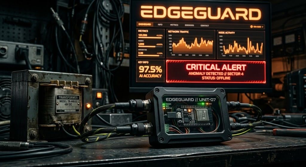
Power transformers are among the most critical assets in electrical distribution infrastructure. Their unexpected failure can result in power outages, safety hazards, equipment damage, expensive repairs, and long service interruptions. Traditional transformer maintenance practices often rely on periodic manual inspection, offline testing, or run-to-failure maintenance. These methods are expensive, slow, labor-intensive, and unable to detect rapidly developing faults in real time. EdgeGuard is an AI-driven, edge-computing predictive maintenance system designed to continuously monitor transformer health and forecast failures before catastrophic damage occurs. The system acts as a retrofittable “Digital Doctor” for distribution transformers by combining low-cost industrial sensors, an ESP32 microcontroller, local intelligence, machine learning-based risk prediction, autonomous relay control, and a real-time web dashboard. The proposed system monitors six major transformer health indicators: temperature, humidity, vibration, oil level, current, and voltage. These signals are normalized and processed through a Multi-Layer Perceptron neural network to classify transformer condition and estimate failure risk. If the predicted risk crosses a critical threshold of 80%, EdgeGuard automatically triggers a relay through GPIO 26 to isolate the transformer from the electrical network. The system also supports secure remote control, dashboard monitoring, API-key-based hardware authentication, JWT-based user access, WebSocket live updates, and automatic live-hardware detection. With an estimated deployment cost of approximately ₹3,850, EdgeGuard offers a low-cost alternative to conventional transformer monitoring systems. Its cloud-independent operation and edge-based decision-making make it especially useful for rural and semi-urban distribution grids where connectivity and maintenance resources are limited.

28 July 2026
ANALYZING TOXIC USER BEHAVIOR AND RISK PATTERNS IN ONLINE GAMING PLATFORMS
This study shows that behavioral data alone can't reliably predict gaming toxicity — but a risk-based model combining behavioral and engineered features does a much better job of flagging the small segment of high-risk users driving disproportionate harm.