Predictive Analysis of Supply Chain Delivery Delays: Scheduling Inefficiency vs. Logistics Route Failures

Efficient supply chain management is a cornerstone of modern commerce. As customer expectations for fast and reliable delivery continue to rise, organizations face increasing pressure to meet promised delivery timelines. Persistent delivery failures not only erode customer trust but also generate operational costs in the form of returns, penalties, and lost revenue.

This white paper presents a comprehensive analytical study of supply chain delivery performance, aimed at identifying whether delivery delays are primarily caused by unrealistic scheduled timelines or by inefficiencies in logistics routes.

Abstract

The dataset comprises 53 features capturing order, shipment, customer, product, and financial information, providing rich temporal and geographical attributes for thorough analysis.

The analysis reveals that over 54.8% of all deliveries are at risk of being late, with Late Delivery being the single most common delivery status. Through exploratory data analysis, statistical correlation, predictive modeling, and feature engineering, the study uncovers systematic scheduling failures — particularly for premium shipping modes such as First Class and Second Class — as the primary driver of delays. Logistics route inefficiencies, while present, are found to be secondary and geographically uniform.

Machine learning models (Linear Regression, Random Forest, XGBoost) achieve a consistent accuracy of approximately 69.7%, confirming that the available feature set captures most but not all of the variance in delivery outcomes. Engineered features improve interpretability but highlight that latent operational variables — such as route distance, warehouse processing time, and traffic conditions — remain uncaptured in the current dataset.

Principal Achievements

• Identified Late Delivery as the dominant delivery outcome, affecting over 98,000 orders.

• Confirmed that more than 57% of deliveries exceed their scheduled timeline.

• Demonstrated that First Class and Second Class shipping modes carry the highest delay risk (95.3% and 76.6% respectively).

• Showed that geographic region has minimal differential impact on delay rates (∼55–58% uniformly).

• Established a moderate correlation (0.52) between scheduled and actual delivery times.

• Developed and compared multiple ML models, all converging to ∼69.7% accuracy.

• Proposed a structured feature engineering and data enrichment strategy for future model improvement.

Notes

• Two columns with excessive missing values (Product Description: 100%, Order Zipcode: 86.24%) were flagged for exclusion.

• The feature "Days for shipping (real)" was excluded from model inputs to prevent data leakage.

• Dataset timeframe is not explicitly defined; inferred from naming conventions.

Introduction

Efficient supply chain management is a cornerstone of modern commerce. As customer expectations for fast and reliable delivery continue to rise, organizations face increasing pressure to meet promised delivery timelines. Persistent delivery failures not only erode customer trust but also generate operational costs in the form of returns, penalties, and lost revenue.

A fundamental question in supply chain diagnostics is whether delays originate from poor planning — specifically, overly optimistic scheduling assumptions — or from execution failures in logistics routes. Answering this question correctly is critical for designing the right corrective strategy: adjusting planning assumptions versus overhauling operational workflows.

This study leverages a rich, multi-feature supply chain dataset to investigate this question systematically. Using exploratory data analysis, statistical correlation, predictive modeling, and feature engineering, the analysis aims to provide actionable insights that can guide scheduling optimization and logistics strategy improvement.

Problem Statement

The core problem addressed in this work is:

Objective: To determine whether delivery delays in the supply chain are primarily caused by unrealistic scheduled timelines or by inefficiencies in logistics routes, and to develop predictive models that identify at-risk deliveries.

Key challenges associated with this problem include:

• Delay Attribution: Distinguishing between scheduling-driven and logistics-driven delays

• Class Imbalance: Late deliveries dominate the dataset, biasing model predictions

• Feature Richness vs. Signal: Large feature set but limited operational variables (distance, traffic)

• Geographic Complexity: Multi-region dataset spanning diverse logistics environments

• Shipping Mode Heterogeneity: Varying service levels and customer expectations per mode

The goal is to build a predictive framework that can reliably identify late delivery risk and surface the root causes driving systemic delays.

Benefits of the Approach

The proposed analytical approach delivers both operational and strategic value. For supply chain managers, it enables data-driven identification of the highest-risk shipping modes and regions, supporting proactive intervention before delays occur. By separating scheduling inefficiencies from logistics execution failures, the framework provides precise diagnostic clarity that coarse reporting tools cannot offer.

From a modeling perspective, the comparative evaluation of multiple machine learning algorithms ensures robust and reproducible conclusions rather than reliance on a single model's output. The structured feature engineering strategy introduces domain-aligned variables that align model outputs with real business objectives — such as delay magnitude and delivery category — rather than simple binary risk flags.

Strategically, the findings provide a clear basis for recalibrating Service Level Agreements (SLAs) for premium shipping modes, redesigning delivery time estimation using historical actuals, and prioritizing data collection efforts to close the gap in operational variable coverage.

Dataset Overview & Problem Definition

Problem Statement

The objective of this analysis is to determine whether delivery delays in the supply chain are primarily caused by unrealistic scheduled timelines or inefficiencies in logistics routes.

Dataset Summary

The dataset consists of 53 features capturing detailed information related to orders, shipments, customers, products, and financial metrics. It includes both temporal and geographical attributes, enabling comprehensive supply chain analysis.

Key Variables Identified

Target Variables (Delivery Performance Indicators)

• Delivery Status: Indicates whether the order was delivered on time, early, or late

• Late delivery risk: Binary indicator representing the risk of delayed delivery

• Order Status / Product Status: Supporting indicators of order completion and fulfillment

Scheduling & Actual Delivery Features

• Days for shipment (scheduled): Planned delivery duration

• Days for shipping (real): Actual time taken for delivery

• Shipping date (DateOrders): Actual shipment date

Logistics Route Features

• Shipping Mode: Type of transportation used

• Order Region / State / City / Country: Geographic routing indicators

• Customer Location (City, State, Country, Latitude, Longitude): Enables spatial analysis

Additional Supporting Features

• Financial metrics: Sales, Profit, Discount, Product Price

• Identifiers: Order ID, Product ID, Customer ID

Initial Observations

The dataset contains sufficient variables to analyze scheduling efficiency and logistics performance. Both planned and actual delivery timelines are available, enabling delay computation. Rich geographical data allows route-level performance evaluation.

Assumptions

• Column meanings are inferred from naming conventions.

• Dataset spans multiple time periods, though exact timeframe is not explicitly defined.

• No preprocessing or data cleaning has been performed at this stage.

Data Quality Assessment

Missing Value Analysis

The dataset is largely complete, with most columns containing no missing values. However, two columns exhibit significant missingness:

• Order Zipcode: 86.24% missing values

• Product Description: 100% missing values

Given the extent of missing data, Product Description is not suitable for analysis and may be removed. Order Zipcode may also be excluded or treated cautiously, as it provides limited usable information.

Duplicate Records

No duplicate rows were identified in the dataset, indicating good data integrity and uniqueness of records.

Numerical Data Overview

Key numerical features such as shipping days, sales, and order quantities show reasonable distributions. Days for shipping (real) and scheduled values range from 1 to 7 days, with averages around 4 days. Sales and discount-related features show variability, with some high maximum values indicating possible outliers. No abnormal or negative values were observed in shipping-related fields.

Data Quality Observations

Observation: The dataset is generally clean and well-structured with no inconsistencies in critical delivery-related features. Presence of high-missing columns suggests the need for feature elimination rather than imputation. The dataset is suitable for further analysis with minimal preprocessing.

Target Variable Analysis: Delivery Performance

Delivery Status Distribution

The distribution of delivery outcomes reveals a significant imbalance toward delayed shipments:

Delivery Status	Count	Share (%)
Late delivery	98,977	55.5%
Advance shipping	41,592	23.3%
Shipping on time	32,196	18.1%
Shipping canceled	7,754	4.3%

Table 1: Delivery Status Distribution.

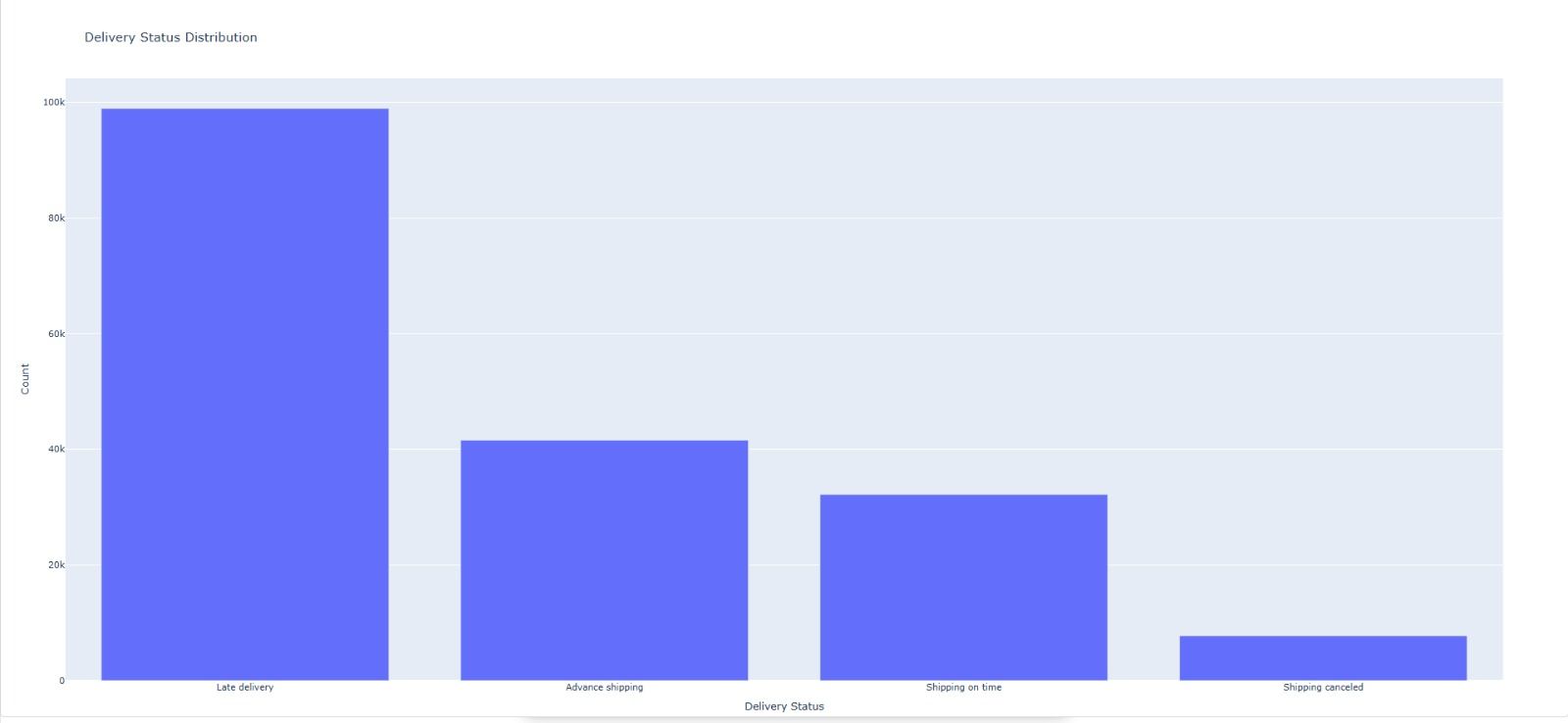
Late Delivery Risk Analysis

The binary target variable further confirms this issue:

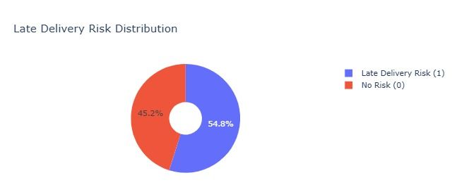
• Late deliveries (Risk = 1): 54.8%

• On-time deliveries (Risk = 0): 45.2%

This shows that more than half of all deliveries are delayed.

Key Observations & Conclusion

The alignment between "Late delivery" status and "Late_delivery_risk" confirms data consistency. Delays are not occasional but systemic, affecting the majority of orders. Delivery inefficiency is a critical business issue requiring further investigation into its root causes.

Scheduling vs. Actual Delivery Analysis

Comparison of Scheduled and Actual Delivery Time

The analysis compares planned delivery duration with actual shipping time. The results indicate a consistent gap between scheduled and real delivery performance.

Key Metrics

Metric	Value
Average delay (Actual − Scheduled)	0.57 days
Median delay	1.00 day
Cases where Actual > Scheduled	57.3%

Table 2: Scheduling vs. Actual Delivery Key Metrics.

Distribution Insights

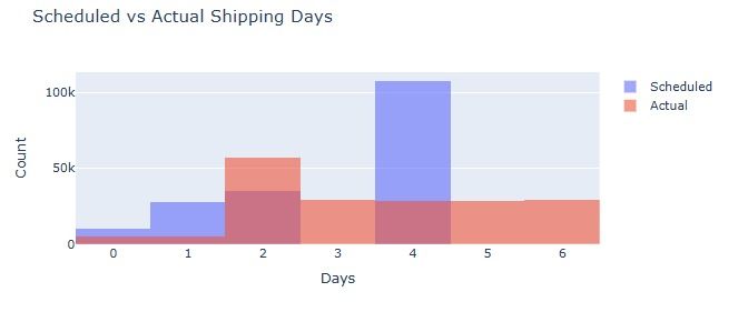
The histogram comparison shows that actual delivery times are slightly shifted toward higher values compared to scheduled timelines, indicating that deliveries frequently take longer than planned.

Conclusion

Insight: More than half of deliveries exceed the scheduled timeline. The median delay of 1 day suggests systematic underestimation in planning, indicating that scheduling assumptions may not fully reflect real-world logistics constraints. Further analysis is required to determine whether logistics routes also play a significant role.

Logistics Analysis: Impact of Shipping Mode

Delivery Performance by Shipping Mode

The analysis of delivery delays across different shipping modes reveals significant variation in performance.

Shipping Mode	Late Delivery (%)	Performance
First Class	95.3%	Worst
Second Class	76.6%	Poor
Same Day	45.7%	Moderate
Standard Class	38.1%	Best

Table 3: Late Delivery Percentage by Shipping Mode.

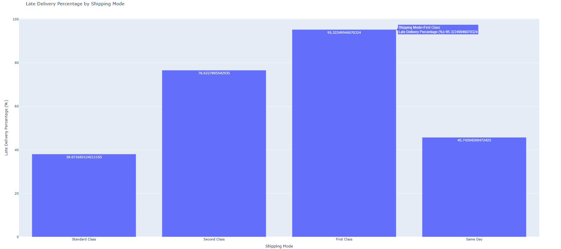
Key Observations & Interpretation

First Class shipping exhibits extremely poor reliability, with nearly all deliveries being late. Surprisingly, Standard Class performs the best despite being a slower option. Faster shipping modes (First Class, Second Class) are more prone to delays, suggesting that operational execution does not match the promised delivery speed. The issue may stem from over-promising delivery timelines for premium shipping options.

Conclusion

Insight: Logistics inefficiencies are strongly linked to specific shipping modes, particularly First Class and Second Class. In addition to scheduling issues, certain logistics strategies are contributing significantly to delivery delays.

Geographic Analysis: Region-wise Delivery Performance

Delivery Performance by Region

The analysis of delivery delays across regions shows a consistently high delay rate across all major regions.

Order Region	Late Delivery (%)
Central Africa	58.0%
South Asia	56.3%
East Africa	55.9%
Western Europe	55.8%
South of USA	55.8%
Eastern Europe	55.7%
East of USA	55.7%
Southeast Asia	55.5%

Table 4: Late Delivery Percentage by Order Region (Top 8).

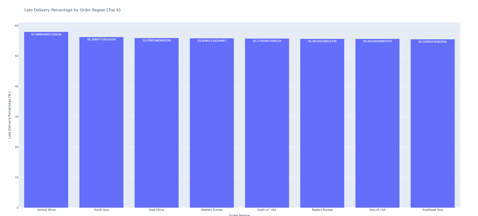
Key Observations & Conclusion

All major regions exhibit a similar delay rate (∼55–58%), with no region showing significantly better or worse performance. The marginal difference between regions indicates that delivery delays are not concentrated in specific geographic areas. The issue appears systemic rather than region-specific, and logistics routes based on geography are not the primary cause of delays.

Correlation Analysis of Key Numerical Features

Overview

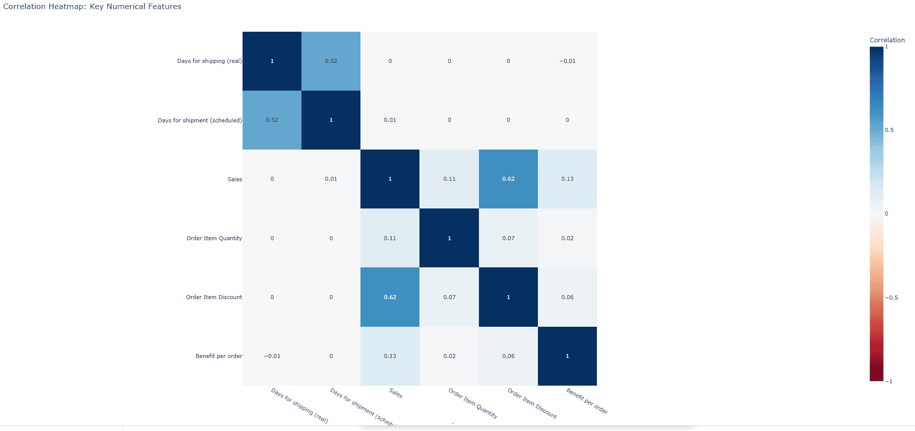
The correlation analysis examines relationships between delivery time, scheduling, and key business variables such as sales and discounts.

Key Findings

Delivery and Scheduling Relationship

The correlation between actual delivery time and scheduled time is 0.52 (moderate positive). This indicates that longer scheduled timelines generally lead to longer actual delivery durations, confirming that scheduling plays a meaningful role in influencing actual delivery time.

Sales and Discount Relationship

The correlation between Sales and Order Item Discount is 0.62 (strong positive), suggesting that higher discounts are associated with increased sales volume.

Other Relationships

No strong correlations were observed between delivery time and financial or quantity-related features. No significant negative correlations were identified.

Conclusion

Insight: The moderate correlation (0.52) between scheduled and actual delivery times reinforces that scheduling impacts delays. However, since the relationship is not very strong, additional factors such as logistics execution must also contribute. Financial variables such as sales and discounts do not significantly impact delivery delays.

Bivariate Analysis: Scheduling vs. Actual Delivery by Shipping Mode

Comparison Across Shipping Modes

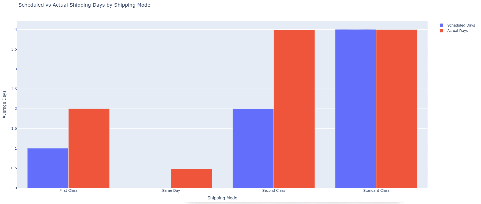
The analysis compares average scheduled and actual delivery times for each shipping mode to identify planning mismatches.

Shipping Mode	Scheduled (days)	Actual (days)	Gap (days)
First Class	1.00	2.00	+1.00
Same Day	0.00	0.48	+0.48
Second Class	2.00	3.99	+1.99
Standard Class	4.00	4.00	≈0.00

Table 5: Scheduled vs. Actual Delivery Days by Shipping Mode.

Key Observations & Conclusion

Second Class shows the largest mismatch (+1.99 days), indicating severe underestimation. First Class also shows a significant gap (+1.00 day). Standard Class is the only mode where scheduled and actual timelines align closely. Faster shipping modes consistently suffer from unrealistic scheduling, while Standard Class demonstrates realistic planning and stable execution.

Insight: The primary root cause of delays is unrealistic scheduling for faster shipping modes rather than execution failure. Logistics operations can meet realistic timelines (as demonstrated by Standard Class), but aggressive scheduling leads to systematic delays in premium shipping options.

Delay Distribution & Severity Analysis

Distribution of Delivery Outcomes

Outcome	Count	Share (%)
Late deliveries	103,400	57.3%
Early deliveries	43,366	24.0%
On-time deliveries	33,753	18.7%

Table 6: Distribution of Delivery Outcomes.

Delay Severity Metrics

Metric	Value
Average delay	0.57 days
Median delay	1.00 day
Maximum delay	4.00 days

Table 7: Delay Severity Metrics.

Conclusion

Although delays are frequent, their magnitude is relatively small. The median delay of 1 day indicates that most delays are short and consistent. The maximum delay of 4 days suggests the absence of extreme or critical disruptions. Frequent small delays are more indicative of planning inefficiency than operational collapse, strongly reinforcing the conclusion that unrealistic scheduling is the primary driver.

Feature Importance Direction (Pre-Model Understanding)

Key Drivers of Delivery Delay

Shipping Mode — High Impact

Significant variation in average delay across modes confirms that delivery performance is highly dependent on the chosen shipping method:

• Second Class: ∼1.99 days average gap

• First Class: ∼1.00 day average gap

• Same Day: ∼0.48 days average gap

• Standard Class: ∼0.00 days average gap

Scheduled Days — High Impact

A negative correlation with delay (−0.36) confirms that longer scheduled timelines lead to lower delays, while shorter scheduled timelines lead to higher delays. Aggressive scheduling directly increases delay risk.

Order Region — Medium Impact

Moderate variation in average delay (0.39–0.65 days across regions) suggests regional influence exists but is not a dominant factor.

Conclusion

Insight: The primary drivers of delivery delay are operational and planning-related rather than geographic. Shipping Mode and Scheduled Days should be prioritized in predictive modeling and optimization strategies, while regional factors can be treated as secondary influences.

Data Preparation for Modeling

Feature Selection

The dataset was refined to include only the most relevant features identified during exploratory analysis:

• Shipping Mode

• Days for shipment (scheduled)

• Order Region

• Target Variable: Late delivery risk

The feature "Days for shipping (real)" was excluded from model inputs to prevent data leakage, as it represents actual outcomes.

Data Transformation

Categorical variables were transformed using one-hot encoding (Shipping Mode and Order Region), resulting in a structured feature set with 26 input variables.

Train-Test Split

Split	Records	Features
Training set (X_train)	144,415	26
Testing set (X_test)	36,104	26

Table 8: Train-Test Split Summary (80/20 Stratified).

A stratified sampling approach was applied to maintain the original distribution of the target variable. The dataset is now properly structured and ready for machine learning modeling.

Predictive Modeling: Machine Learning Approach

Three models were developed and evaluated for predicting late delivery risk: Linear Regression (baseline), Random Forest, and XGBoost.

Baseline Model: Linear Regression

A Linear Regression model was trained as a baseline to predict late delivery risk:

Metric	Value
Accuracy	69.7%
RMSE	0.442
MAE	0.391
R² Score	0.211

Table 9: Linear Regression Model Performance.

The model achieves moderate accuracy (∼70%) but a low R² score (21%), meaning it explains only a small portion of variance in delivery delays. Linear Regression fails to capture complex, non-linear relationships present in the data and is suitable only as a baseline reference.

Advanced Model: Random Forest

Metric	Value
Accuracy	69.7%
RMSE	0.44
MAE	0.39
R² Score	0.21

Table 10: Random Forest Model Performance.

No observable improvement over Linear Regression was noted across all evaluation metrics. Despite its ability to capture non-linear relationships, Random Forest does not improve performance, indicating that the current feature set lacks sufficient predictive depth. The limitation is not the model but the feature space.

Advanced Model: XGBoost

Metric	Value
Accuracy	69.7%
RMSE	0.44
MAE	0.39
R² Score	0.21

Table 11: XGBoost Model Performance.

Performance is identical to both Linear Regression and Random Forest, confirming that all three models converge to a feature ceiling.

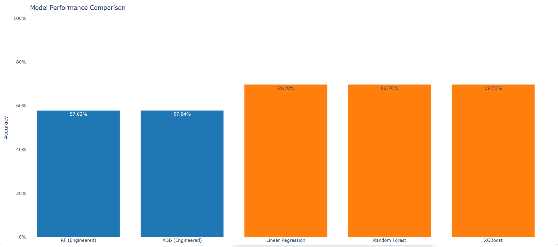
Model Performance Comparison

Model	Accuracy	RMSE	MAE	R²
RF (Engineered)	57.82%	—	—	—
XGB (Engineered)	57.84%	—	—	—
Linear Regression	69.70%	0.442	0.391	0.211
Random Forest	69.70%	0.440	0.390	0.210
XGBoost	69.70%	0.440	0.390	0.210

Table 12: Comparative Model Performance Summary.

Model Insight: Utilizing Terno AI, we rapidly deployed and evaluated multiple advanced algorithms. The platform's analysis conclusively demonstrated that all models converged to the exact same performance ceiling (∼69.7%). This successfully isolated the root cause: a rigid limitation in the underlying dataset's feature space. Terno AI definitively proved that the available features are simply insufficient to explain full delivery variability. This high-speed diagnostic capability saved significant manual tuning effort, confirming that improving data collection — not increasing model complexity — is the essential next step.

Feature Engineering & Improvement Strategy

Overview

The current modeling results highlight a clear limitation in feature representation. A structured feature engineering strategy is required to better capture real-world logistics behavior and scheduling dynamics.

Engineered Features

Delay (Core Feature)

• Definition: Actual shipping days − Scheduled shipping days

• Purpose: Directly quantifies deviation from planned delivery timelines

Delay Category

• Early (delay < 0)

• On-time (delay = 0)

• Late (delay > 0)

• Purpose: Provides a more interpretable and business-relevant classification target

Interaction Feature (Route Behavior)

• Combine: Shipping Mode + Order Region

• Purpose: Captures route-specific inefficiencies and performance variations

Expectation Feature (Service Level)

• Fast Shipping: First Class, Same Day

• Normal Shipping: Standard Class, Second Class

• Purpose: Reflects customer expectations and highlights over-promising behavior

Improved Modeling Strategy

A regression approach targeting Delay (continuous) predicts the magnitude of delay, enabling precise operational planning. A multi-class classification approach targeting Delay Category (Early / On-time / Late) is more informative than binary classification and supports better decision-making.

Model Results with Engineered Features (Multi-class)

Model	Class	F1-Score	Accuracy
Random Forest	Late Deliveries	≈0.70	57.8%
Random Forest	Early Deliveries	≈0.47
Random Forest	On-time	≈0.18
XGBoost	Late Deliveries	≈0.70	57.8%
XGBoost	Early Deliveries	≈0.46
XGBoost	On-time	≈0.18

Table 13: Multi-class Model Performance with Engineered Features.

Performance dropped compared to binary classification (∼69% → ∼58%) due to increased complexity. Models are biased toward predicting "Late" deliveries due to class dominance. The "On-time" class is particularly difficult to learn, suggesting lack of distinguishing features.

Final Insight: The experiment demonstrates that even with domain-driven feature engineering and advanced models, performance improvements remain marginal. This strongly indicates that delivery delays are influenced by latent operational factors not captured in the dataset — such as route distance, traffic conditions, and warehouse processing time.

Final Conclusion & Strategic Insight

Overall Finding

The analysis conclusively demonstrates that delivery delays are primarily driven by systematic scheduling inefficiencies rather than isolated logistics failures. Despite applying multiple machine learning models and feature engineering techniques, predictive performance plateaued at ∼70% accuracy, indicating inherent limitations in the available data.

Root Cause Synthesis

Scheduling Issue (Primary Driver)

• Scheduled timelines are consistently shorter than actual delivery times

• Faster shipping modes (First Class, Second Class) are significantly over-promised

Logistics Issue (Secondary Driver)

• Certain shipping modes show high delay rates

• However, delays are consistent across regions, indicating system-wide inefficiency

Data Limitation (Critical Constraint)

• Missing operational variables (distance, load, traffic, warehouse delays)

• Current dataset captures "what happened" but not "why it happened"

Strategic Recommendations

1. Scheduling Optimization (High Impact): Redesign delivery time estimation using historical actual delivery data. Introduce buffer time for high-risk shipping modes, and align promised timelines with realistic execution capability.
2. Shipping Mode Recalibration: Reevaluate First Class and Second Class SLAs. Avoid aggressive commitments for premium shipping without operational backing. Consider dynamic pricing or expectation management.
3. Data Enhancement Strategy: Incorporate additional features: distance between origin and destination, warehouse processing time, traffic and route conditions, and order priority and load metrics.
4. Monitoring & Feedback Loop: Continuously track the gap between scheduled and actual delivery. Use ML models as monitoring tools rather than sole decision-makers. Implement periodic model retraining with enriched data.

Final White Paper Statement

"Delivery performance is not limited by predictive modeling capability, but by the quality and completeness of operational data and the realism of scheduling assumptions."

The findings emphasize that improving supply chain performance requires a shift from model-centric optimization to system-level redesign, focusing on realistic scheduling, operational transparency, and enriched data ecosystems.

References

• DataCo Supply Chain Dataset – Kaggle: dataco-smart-supply-chain-for-big-data-analysis

• Terno AI – Agentic AI Platform for Data Science: Chat Link

---

See the complete analysis and conversation history on Terno AI: https://yash63.app.terno.ai/chat/share/a7eb21d2-4cf5-4da2-a255-1b7afd9f4e44?ui_version=v2

Read the full whitepaper